Dataverse Conditional Access & MFA: Enterprise Auth Strategy Without Breaking Power Platform

You’ve mandated that your organization must enforce conditional access policies and multi-factor authentication across all cloud services. It’s the right call from a security standpoint. Your CISO is demanding it, your compliance framework requires it, and your risk assessment puts it at the top of the priority list.

But then you hit the wall: conditional access policies that work perfectly for Microsoft 365 web applications cause Power Platform apps to stop authenticating altogether. Users can no longer access the Power Apps that run critical business processes. Your integration flows in Power Automate start failing because they’re hitting MFA challenges mid-workflow. The Dataverse API connections that your Line of Business applications depend on suddenly require interactive authentication that isn’t available in batch processing scenarios.

The tension isn’t theoretical. It’s real, it’s urgent, and it forces you to choose between security governance and operational continuity. Most organizations resolve this tension by weakening their conditional access policies, carving out exceptions for Power Platform, or exempting service accounts from MFA entirely. All of those choices push you further from true security maturity.

There’s a better path, but it requires understanding how Dataverse, Conditional Access, and the Power Platform authentication layer actually interact.

Why Standard Conditional Access Policies Break Power Platform

Conditional Access is a powerful feature in Azure AD. It evaluates device compliance, sign-in risk, geographic location, and dozens of other signals before granting authentication tokens. When you create a policy that requires MFA for all cloud apps, or limits access to corporate-managed devices, you’re making a sound security decision.

The problem: Power Platform applications don’t authenticate the same way that Outlook or SharePoint do.

When a user opens Power Apps in a browser, they’re presented with an interactive login page. That interface can handle MFA prompts, device compliance checks, and the full conditional access flow. So far, so good. But many organizations use Power Apps in ways that don’t involve a browser:

  • Mobile apps built on Power Apps don’t always gracefully handle MFA challenges in the middle of a user session.
  • Service accounts that run cloud flows in Power Automate are trying to authenticate without user interaction, which violates the interactive requirement of most conditional access policies.
  • Custom applications that use the Dataverse Web API through a service principal must request tokens in a non-interactive context. If your conditional access policy requires MFA or device compliance checks, the token request fails.
  • Integration scenarios where your on-premises LOB application authenticates directly to Dataverse hit the same wall.

The Dataverse API itself doesn’t block these scenarios. Azure AD’s conditional access policies do. The authentication platform is saying, “I need interactive user presence to validate MFA,” but the application doesn’t have a way to provide it.

The Real Cost of Over-Exempting Service Accounts

When token requests fail, the most common workaround is to exempt service accounts from conditional access policies. If you carve out an exclusion for all accounts in a particular group, those accounts no longer need to satisfy MFA requirements, even though their access might be just as sensitive as any human user’s.

This creates a security problem that goes deeper than it first appears:

First, service accounts become targets. If a threat actor gains access to a service account password, they have a golden ticket to your Dataverse environment without triggering MFA challenges. They can run integration flows, extract data, or modify records in batch operations that are harder to detect than interactive user activity.

Second, the exemption tends to expand over time. One service account becomes two. Two becomes five. Then you’re exempting entire groups. The exception becomes the rule, and your conditional access policy devolves into a symbolic gesture rather than a functioning security control.

Third, you lose the audit trail. When a service account isn’t subject to conditional access policies, you don’t get the same visibility into what it’s doing. Azure AD doesn’t log conditional access evaluations for exempt accounts. Your security team can see that the account authenticated, but not whether it was accessing data from an expected location, or whether the request exhibited anomalous characteristics.
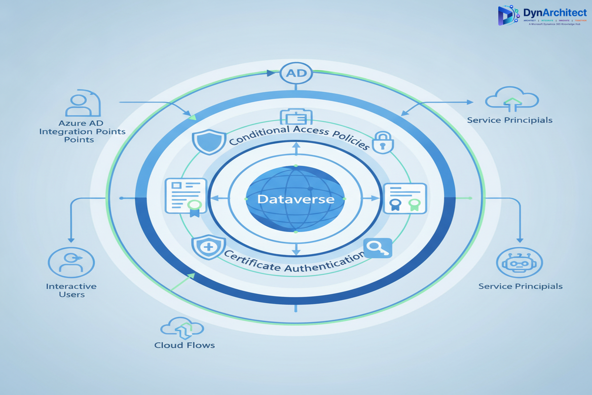
Implementing Conditional Access for Power Platform Without Breaking Applications

The solution requires thinking about service accounts, Power Apps clients, and Dataverse API access as three distinct authentication scenarios, each with different architectural requirements.

Scenario 1: Interactive Power Apps and Power Automate Usage

This is the easiest scenario to secure. When a user opens Power Apps or Power Automate in a browser, they’re in an interactive context. Standard conditional access policies apply directly. You can require MFA, enforce device compliance, and apply geographic restrictions without breaking the user experience.

The key is to ensure that your Power Apps environment is registered in Azure AD as a cloud application, and that conditional access policies explicitly include it. Many organizations assume that Power Apps are covered by broad policies that target “all cloud apps,” but Power Apps needs explicit mention in the policy scope.

For Power Automate, the situation is slightly different. Cloud flows that require user interaction can handle MFA. But the moment you implement a background cloud flow, you’re in a non-interactive context. Conditional access policies that require MFA will block the token request.

Scenario 2: Unattended Cloud Flows and Service Accounts

This is where most organizations struggle. A cloud flow that processes orders, sends notifications, or synchronizes data is running without a user present. It needs a way to authenticate to Dataverse without triggering an MFA challenge.

The recommended approach is to use a managed identity or a service principal with a certificate-based credential, combined with a conditional access policy that evaluates non-interactive sign-ins differently than interactive ones. Instead of requiring MFA for all accounts, your policy should:

  • Require MFA for interactive sign-ins from all user accounts.
  • Skip MFA for service accounts or managed identities, but enforce stronger authentication (certificate-based credentials instead of passwords).
  • Apply additional controls to service accounts, such as restricting geographic locations or requiring authentication from specific networks.

The idea is that MFA is one control among many. If you compensate for the absence of MFA with other controls (certificate authentication, network restrictions, IP allowlisting), you maintain a strong security posture without blocking legitimate application access.

Scenario 3: Custom Applications and Direct Dataverse API Access

When a Line of Business application calls the Dataverse Web API directly, it’s requesting a token using application credentials. This is always a non-interactive flow. Conditional access policies that block non-interactive sign-ins will block this access.

Here’s where conditional access policies designed for interactive users start to feel restrictive. Your policy might say “Require MFA and a corporate device,” but neither condition can be evaluated for a non-interactive application. You’re forced to choose between blocking the integration or exempting the service account.

The better solution is to use a service principal with certificate-based authentication, combined with conditional access policies that allow certificate-authenticated service accounts to authenticate without MFA, but apply other compensating controls: network-based restrictions, role-based access control, and comprehensive audit logging.

Designing the Authentication Flow

Here’s how to architect this at the enterprise level:

Step 1: Segment Your Conditional Access Policies by Sign-In Type

Create two distinct conditional access policies: one for interactive sign-ins and one for non-interactive sign-ins. The interactive policy can be strict (require MFA, device compliance, geographic restrictions). The non-interactive policy should be more lenient on the authentication factor, but compensate with additional controls.

Step 2: Use Certificate-Based Credentials for Service Principals

Never use passwords for service accounts that need to authenticate to Dataverse. Certificates are more secure, easier to rotate, and compatible with conditional access policies that distinguish between interactive and non-interactive flows.

Step 3: Implement Network-Based Restrictions

Use conditional access policies to restrict service accounts based on network location. If your integration platform is running on premises, create a policy that allows your service principal to authenticate only from that server’s IP address. This adds a layer of security: even if credentials are compromised, the attacker can’t authenticate from an arbitrary location.

Step 4: Enable Comprehensive Logging and Monitoring

Enable Azure AD sign-in logs and audit logs. Monitor for sign-in failures, authentication attempts from unexpected locations, large batch operations, and privilege elevation. Use Azure Sentinel or a SIEM to correlate these signals and alert on anomalous activity.

Step 5: Test and Validate Before Enforcement

Before enforcing conditional access policies broadly, test them with your Power Platform applications, integrations, and service accounts. Use the conditional access policy’s report-only mode to see which authentication attempts would be blocked, then adjust policies to allow legitimate scenarios.

Implementation Challenges and How to Avoid Them

Challenge 1: Power Apps and Power Automate Have Different Requirements

Power Apps desktop application, mobile apps, and cloud flows each have slightly different authentication behavior. Test each scenario in your environment.

Challenge 2: Certificate Rotation Is Easy to Forget

Service principals with certificate-based credentials need regular rotation, typically every 1 to 2 years. Implement automated certificate rotation using Azure Automation or App Service certificate management.

Challenge 3: Conditional Access Policies Interact With Each Other

If you have multiple policies, they’re all evaluated. A token request must satisfy all applicable policies. Regularly review your policy set and consolidate where possible.

The Path to Zero Trust

Implementing conditional access and MFA for Power Platform and Dataverse is a step toward Zero Trust security architecture. Instead of trusting an account because it has MFA enabled, you trust accounts based on multiple signals: device state, location, authentication method, audit trail, and runtime behavior.

For Dataverse environments that handle sensitive data or run mission-critical processes, this level of security maturity is essential. The key is to design your authentication architecture around your actual use cases, not around a generic policy that exempts half your accounts.

Your CISO wants to see conditional access and MFA enforced. Your application owners need Power Platform and integrations to work reliably. These goals aren’t in conflict if you architect the authentication layer thoughtfully.


Configuring Field Service Requirement Groups Before You Turn On the Scheduling Operations Agent

Field service dispatcher reviewing a multi-resource schedule board on a large monitor

A dispatcher at a commercial HVAC contractor gets a work order for a rooftop unit replacement that needs a refrigerant-certified technician and a licensed electrician on site at the same time. Neither one can do the job alone, and the customer has a four-hour access window. On most schedule boards, this becomes two separate booking searches, two different sets of availability to cross-reference by hand, and a fair amount of guessing about who else is nearby when the first match falls through. Dynamics 365 Field Service has had a purpose-built answer to this for a while, and it lives inside a feature called Field Service requirement groups. What changes this year is that Field Service is also rolling out an AI agent that can optimize those multi-resource schedules on its own, and the two capabilities need to be understood together, not separately, if a rollout is going to hold up.

Field service dispatcher reviewing a multi-resource schedule board on a large monitor

Why Requirement Groups Exist

A requirement group bundles several resource requirements that are commonly scheduled together for a single job: two technicians with different skills, a technician paired with a piece of equipment, or a facility resource alongside the staff member who runs it. It solves a narrower problem than it sounds like it should. Field Service already has crews for resources who always work as a fixed unit, so requirement groups are reserved for combinations that vary from job to job, which is exactly the HVAC scenario above. Get that distinction wrong early and dispatchers end up maintaining crew records for what are really one-off pairings, which defeats the purpose of either feature.

Configuring Field Service Requirement Groups: A Three-Step Setup

Building a usable requirement group takes three steps, and the order matters more than the documentation implies, because the template governs everything downstream.

The first step is the requirement group template, created under Resource Scheduling settings. Two fields here decide how strict the matching logic is. The “Select” setting is either All, meaning every resource in the group must satisfy every requirement, or Any, meaning a resource can fulfill any one of them; nesting subgroups lets a team combine both, for instance a root group set to Any with two subgroups each set to All, which is how a dispatcher models “either an electrician-plus-tech pairing or a single dual-certified tech will do.” The “Part of Same” setting controls how tightly the resources have to be related to each other, ranging from a shared location association up through a shared organizational unit, which is the strictest option and the one most enterprises with multiple legal entities or regional service territories will actually need.

The second step is adding individual requirements to the template: duration, characteristics or skills, resource categories, work location (facility, on-site, or location-agnostic), and preferred resources, each capped at ten values. That cap is easy to hit for a services company with a large skills taxonomy, and the practical fix is to push filtering down to characteristics rather than trying to enumerate every acceptable technician by name.

The third step is booking through the schedule assistant, which searches for resources that can fulfill the group’s requirements and defaults to recommending the option requiring the fewest resources first. Requirement group templates can also be attached directly to incident types, so a work order created from a known incident type pulls in its multi-resource requirements automatically instead of relying on a dispatcher to remember which jobs need a paired booking.

The Detail That Breaks Onsite Jobs

One behavior catches teams off guard during go-live. The schedule assistant matches resources by arrival time, not by when they start traveling. For a job where both resources are dispatched from the same depot, that distinction rarely matters. It matters a great deal when one technician is thirty minutes from the site and the other is ninety minutes out on a different route; the assistant will still try to land them at the customer’s door at the same moment, which can mean the closer resource sits idle waiting for a window that a smarter dispatcher would have staggered. Any territory with technicians spread across a wide radius should account for this when setting expectations with dispatch staff, rather than treating a rejected recommendation as a bug.

A handful of other constraints are worth knowing before they show up as a production surprise. Requirement groups do not support multi-day scheduling; a job spanning more than one day needs Field Service’s separate multi-day scheduling capability instead. Every requirement inside a group must share the same duration, so a job needing a technician for four hours and a specialist for only the first hour has to be modeled as two bookings, with cascade crew changes disabled afterward so adjusting one booking’s length does not silently drag the other along with it. And incident types that already carry their own characteristics cannot be linked to a requirement group template at the same time, which pushes teams toward attaching characteristics to the individual requirements inside the group rather than to the incident type itself.

Two field service technicians consulting a tablet showing work order and scheduling details

Where the Scheduling Operations Agent Fits

Requirement groups solve how a multi-resource job gets modeled and booked once. The Scheduling Operations Agent, entering broader preview this month, is aimed at a different problem: keeping the whole day’s schedule coherent after the first booking, when cancellations, overruns, and priority changes start cascading across a technician roster. It already handled single and multi-resource optimization in an earlier preview; what is new is an “automate optimizations” capability that runs in two modes. Interactive mode surfaces suggested changes for a dispatcher to accept in the moment, which is closest to how the tool has worked so far. Batch mode runs asynchronously against a defined scope of resources, on a schedule, which is the part that actually reduces manual dispatch work rather than just speeding up the click-through.

The naming is a little ahead of what the feature currently does, and that gap is worth being precise about with stakeholders. Every optimization the agent proposes, in either mode, still requires human approval before it takes effect, and it will not touch a booking marked “Do Not Move.” That is a sensible guardrail, but it means batch mode is closer to an overnight queue of pre-vetted suggestions waiting for a morning review than to unattended rescheduling. Teams evaluating this as a way to cut dispatcher headcount should model it as an efficiency gain on the review step, not a removal of the step.

Setup runs through three admin-configured objects: goals, which define what the agent is optimizing for and the constraints it has to respect, such as skill eligibility and territory boundaries; scopes, which define which resources and requirements are in play; and plans, which schedule batch runs. None of this is exposed to end users by default, so a pilot needs a maker or admin to own the configuration from day one, and it needs a data foundation of accurate characteristics and territory assignments on the underlying resources, since the agent’s recommendations are only as good as the constraint data it is reading. This is also where requirement group discipline pays off twice: a schedule with sloppy or missing characteristics will produce weak optimization suggestions regardless of how well the agent itself is configured. Regional rollout is uneven as well; the feature is unavailable in Azure Government and China cloud environments and is still expanding across other regions, so a multinational deployment should confirm coverage before promising a go-live date to any specific site.

Sequencing a Rollout That Actually Holds

The practical order is to get requirement groups and their underlying characteristics right first, on a defined subset of incident types, before layering the agent on top. A team that tries to configure both at once tends to spend its pilot debugging which layer produced a bad recommendation. Once requirement group bookings are reliable for a specific service line, interactive-mode agent suggestions are a reasonable next step, since a dispatcher is reviewing every change anyway. Batch mode is worth piloting only after that interactive period has built some trust in the agent’s judgment on that same resource pool, and even then it should start on a narrow scope rather than the full technician roster. Routeget Technologies has run this kind of phased rollout with field service clients who tried to skip straight to full automation and ended up rebuilding their characteristic taxonomy mid-project instead; sequencing it the other way costs a little more calendar time upfront and considerably less rework later.


#FieldServiceScheduling #RequirementGroups #SchedulingOperationsAgent #MultiResourceBooking #DispatchOptimization #DynamicsFieldService

Why Your Supply Chain Visibility Stops at Your Warehouse Door: Building End-to-End Traceability in Dynamics 365

Why Your Supply Chain Visibility Stops at Your Warehouse Door: Building End-to-End Traceability in Dynamics 365

It’s 2 a.m. on a Tuesday. Your manufacturing facility just identified a critical defect in raw materials that arrived from a supplier last week. By the time your quality team finished root-cause analysis, those defective materials were already processed into three separate production batches. Now you’re facing potential customer recalls, regulatory notification deadlines, and no clear way to trace which finished goods actually contain the defective material. Your supply chain software told you where the raw material was ordered and when it arrived. It told you absolutely nothing about where it went after that.

This scenario plays out in manufacturing and distribution operations every day. Supply chain visibility systems excel at tracking inbound inventory but break down once materials enter production or move through fulfillment. For many operations leaders, the supply chain becomes a black box the moment inventory leaves the warehouse.

The business cost of that blind spot is substantial. When quality issues surface, traceability delays mean either expensive and conservative recalls that pull good products from shelves, or risky decisions to ship products you cannot confidently verify as safe. For regulated industries, regulators expect faster, more precise responses than manual investigation can deliver. Beyond quality, lost visibility into material flow makes it nearly impossible to understand true landed costs, verify supplier performance claims, or negotiate accurately on future contracts.

Dynamics 365 Supply Chain Management addresses this visibility gap by connecting procurement, inventory, production, and fulfillment into a unified traceability architecture. The difference is not just better information. It is speed and precision when those information gaps cost you the most.

The Visibility Problem Runs Deeper Than Poor Reporting

Most supply chain systems treat traceability as an optional feature bolted onto inventory management. A truck arrives with materials. The system records receipt and location. Then it moves to the next transaction. There is no continuous thread connecting that receipt to the production order that consumed it, to the manufactured batch that contains it, to the shipment that sent it to customers.

This architectural gap exists because legacy systems were built for transaction volume, not data continuity. A system designed in 1997 needed to process thousands of purchase orders and shipments daily. It could not afford to maintain detailed linkages between every input and output. Instead, operations relied on physical batch logs, manual tracking spreadsheets, and the assumption that anyone who needed to trace materials would do so through paper records and institutional memory.

That model breaks when scale grows, when complexity increases, and when regulators start asking for proof instead of accepting your word.

The actual impact shows up in three ways. First, quality investigations take weeks instead of days because tracing backward from a customer complaint requires manual detective work across multiple systems and warehouses. Second, compliance teams spend months preparing for audits because they cannot quickly demonstrate that materials flowed exactly as regulations require. Third, cost analysis remains vague because you cannot match specific materials through production to specific finished goods and actual profit margins by customer or product line.

For operations leaders evaluating the business case for new systems, this is the tension: your current software works fine for running day-to-day operations, but it leaves you strategically blind when problems surface.

Dynamics 365 Solves This Through Persistent Tracking Dimensions

Dynamics 365 Supply Chain Management addresses traceability through a concept called inventory tracking dimensions. These are optional attributes you assign to materials when they arrive that the system carries forward through every downstream transaction.

In practice, this means when a raw material shipment arrives from a supplier, you can assign a lot number, a batch identifier, or a supplier batch code to that inventory. Every time that material moves, Dynamics 365 maintains that linkage. When it gets consumed in production, the system knows exactly which finished goods batch contains that material. When the finished goods shipment occurs, the system knows which supplier lot reached which customer.

This is simpler than it sounds in theory and more complex in execution. The traceability chain only works if data quality is maintained at every step. Warehouse receiving teams must accurately record lot numbers when materials arrive. Production schedulers must use the right lot allocation logic so materials move in the order and combinations you intend. Finished goods picking must respect lot traceability so batches do not inadvertently mix material from multiple suppliers.

Beyond receiving and production, Dynamics 365 extends visibility into logistics through Transportation Management integration. When finished goods ship, the system can attach the upstream supplier and production batch information to the shipment record. If your logistics partners accept real-time shipment data, you can even extend visibility beyond your own dock to show customers or regulators exactly when and how products moved from your facility.

Quality management workflows layer on top of this. When a quality hold is placed on a supplier lot, Dynamics 365 can automatically flag all downstream inventory and production batches that contain that material. Recalls, when they become necessary, can be precisely scoped to affected batches rather than conservative over-recalls of everything you cannot immediately rule out.

The Implementation Reality

Building this capability requires more than buying software. It requires operational discipline and often represents a genuine change in how warehouse and production teams work.

First, data quality becomes non-negotiable. If lot numbers are not recorded accurately at receiving, the entire chain breaks. Many organizations find this is the hard part, not the technology. Warehouse teams accustomed to checking boxes now need to record specific identifiers and understand why precision matters. For operations leaders, this means investment in training and ongoing quality checks, not just software implementation.

Second, integration with logistics partners becomes necessary if you want visibility to extend beyond your facility. Most transportation management systems now accept data feeds, but the integration requires coordination and often custom mapping to match your identifier schemes with your logistics partners’ systems.

Third, implementation timelines are usually longer than initial estimates because the visibility you gain surfaces data quality issues that existing systems were hiding. You may discover that your receiving team has been using approximate lot numbers or that production scheduling has been commingling materials from different lots without clear documentation.

For most mid-market to large manufacturers, the return on investment justifies that effort. Once you have consistent end-to-end traceability, quality investigations that previously took ten business days now take one. Compliance audits shift from defensive documentation gathering to straightforward system queries. Supplier negotiations become evidence-based rather than assumption-based when you can show precisely how their material performed through your production process.

What This Means for Your Supply Chain Strategy

The businesses that maintain the strongest competitive positions today are those that treat supply chain as a strategic asset, not a cost center. Part of that strategy is building the visibility to know what you own, where it is, and what happened to it at every stage.

Dynamics 365 Supply Chain Management makes that visibility achievable at reasonable scale. The foundation is simple: persistent tracking dimensions that follow materials from receipt through production and shipping. The execution requires discipline and investment in data quality and integration. The payoff is speed and precision when quality issues surface, confidence in regulatory readiness, and the data you need to make supplier performance and profitability decisions based on fact instead of intuition.

If your current supply chain software has a blind spot after inventory leaves the warehouse, that blindness has a cost. The question is whether you measure it.


#SupplyChainTraceability #Dynamics365SCM #InventoryTracking #SupplyChainVisibility #LotTracking #QualityManagement #SupplyChainCompliance #ManufacturingERP

Business Central Production Scheduling: Why Visual Scheduler Configuration Fails When Demand Patterns Change

Production scheduling in Business Central sounds straightforward until you implement it at scale. The visual production scheduler promises drag-and-drop job sequencing and real-time capacity planning. Deploy it and discover that your demand patterns don’t fit the assumptions the system bakes into its default behavior. Planners revert to spreadsheets within weeks. The scheduler wasn’t broken; the configuration was incomplete.

The visual production scheduler in Business Central sits between shop floor execution and demand planning. It maps jobs to work centers, respects capacity constraints, and surfaces bottlenecks visually. But it works only when three conditions align: demand forecasts are stable, work center capacity is fixed, and job dependencies follow predictable patterns. Change any one of those, and the scheduler either produces schedules that don’t work or gets abandoned for manual planning.

Why Visual Scheduling Breaks Under Real Demand

Most implementations configure the scheduler once at go-live, assume demand won’t shift significantly, and leave it. Demand does shift. Seasonal patterns emerge. Customers request expedited jobs. Supply constraints force substitution of materials that process differently. The visual scheduler has no feedback loop; planners see outdated capacity assumptions in their schedules but have no way to tell the system that the underlying model has changed.

The core issue is that the scheduler operates on historical work center capacity and fixed routing assumptions. When a customer order arrives that doesn’t match the standard bill of materials or when a work center consistently underperforms its configured hours available due to changeover time or quality hold-ups, the scheduler still assumes standard capacity. Planners know the real constraint (the paint booth runs six hours a day, not eight, because of cure time between jobs), but the system doesn’t. Schedules become fiction.

Adding seasonality creates a secondary failure mode. Winter orders require different sequencing than summer demand. Heat-treating capacity bottlenecks shift based on product mix. The scheduler can’t recognize these seasonal patterns because configuration is static. A planner building schedules manually can say, “December through February, we prioritize thinner stock because it moves through coating faster.” The visual scheduler just sees jobs and available hours and proposes sequences that look optimal on the Gantt chart but fail in execution.

The Configuration Reality

Setting up the visual scheduler correctly requires knowing your capacity model in detail before you have execution data. That’s the uncomfortable truth. You need to define work center hours, parallel or sequential capacity, setup and teardown time, quality hold periods, material feed time, and routing flexibility. Get any of those wrong, and schedules drift immediately from what the system proposes to what planners can actually execute.

Most small and medium manufacturers don’t have this data documented at configuration time. They know their shop floor, but they don’t have it formalized into the work center master in Business Central. So they estimate. The estimates are close but not exact. Schedules are therefore slightly off from day one. The delta is small enough that planners don’t notice for weeks, but once they do, credibility in the tool evaporates.

Diagnosis: When Schedules Stop Matching Reality

The failure usually manifests as a mismatch between what the scheduler says can be done and what actually ships. A planner creates a schedule showing three jobs fitting into a work center in a day. The first job completes on time, but the second never starts because the first consumed more setup time than the system assumed. The planner gets blamed for a bad schedule. The scheduler gets blamed for being unrealistic. Neither blame is accurate; the system doesn’t know the real setup time.

Spot this problem early by comparing historical throughput data against scheduler assumptions. Pull actual shop floor execution history and overlay the capacity assumptions in each work center definition. If real throughput is 15 percent lower than configured, the system is optimistic. If throughput is 15 percent higher, the system is conservative (less common, but it happens when planners are very efficient or when the scheduler’s assumptions about parallel work are overstated). The gap is your calibration opportunity.

Three Production-Ready Fixes

The most effective fix is to build a demand-responsive scheduling loop. Instead of assuming demand is stable, capture actual demand patterns over a rolling window (usually 3-6 months of order data) and re-baseline the scheduler assumptions quarterly or semi-annually. This doesn’t require expensive plugins; it requires discipline in the operations team to review throughput variance and update work center capacity definitions when patterns change.

Second, implement a hierarchical scheduling approach. Use the visual scheduler for the primary constraint (often one critical work center) and leave everything else to manual planning or automated sequencing. Don’t try to optimize the entire job shop simultaneously; optimize the bottleneck. Everything else sequences around it. This reduces the configuration surface and makes the system more robust to planning changes.

Third, establish a feedback cycle between planners and the master scheduler. Every two weeks, have the planner who lives with the schedule review it and flag five jobs that were either much easier or much harder to execute than the system predicted. Feed those observations back into work center definitions. This is operational overhead, but it’s the operational overhead that keeps the scheduler aligned with reality instead of chart fantasy.

When to Accept Spreadsheets Instead

Not every manufacturer can or should use the visual scheduler. If your demand patterns change weekly, your jobs have highly variable routing, or your work centers have truly shared capacity across unrelated product families, the scheduler will always lag reality. In those cases, accept that planners will use spreadsheets or written job cards and build Business Central to support that workflow. Track scheduled completion dates and actual completion dates, but don’t pretend a static scheduler will optimize a fundamentally dynamic shop floor.

For manufacturers with repeatable products, stable demand patterns, and one or two clear bottlenecks, the scheduler is valuable. For job shops or custom manufacturers, it’s decoration.

Moving Forward

The visual production scheduler in Business Central is a tool, not a solution. It works best when you know your constraints and keep them documented. It fails quietly when assumptions drift from reality without anyone noticing until schedules stop matching execution. The organizations that sustain scheduler use treat it as a system that needs constant calibration, not a one-time configuration.

Start with the simplest possible scheduler setup: one work center, one product family, one demand pattern. Get that right before adding complexity. Use the first three months of data to calibrate. Then decide whether to expand or whether your planners are already doing a better job with their current method and the scheduler will just slow them down. That’s the conversation that happens too late in most implementations, when the scheduler is already abandoned.

About Routeget Technologies: With over a decade of Business Central implementation experience across discrete, process, and hybrid manufacturers, Routeget helps organizations design production planning systems that planners actually use. Our consultants focus on aligning system configuration with operational reality rather than forcing operations to match system assumptions.


#BusinessCentralManufacturing #ProductionScheduling #ManufacturingERP #JobShopScheduling #CapacityPlanning #BusinessCentral #SupplyChainOptimization #SmallManufacturing

Implementing Robust Error Handling in Power Automate: Patterns for Enterprise Deployments

One of the most insidious threats to enterprise automation is the silent failure—a workflow that appears to complete successfully but delivers corrupted data, skipped steps, or incomplete transactions. In Power Automate, uncaught errors compound this risk when operations fail without proper logging or recovery mechanisms. Implementing robust error handling isn’t just best practice; it’s essential infrastructure for reliable cloud automation.

Enterprise deployments demand structured, predictable error handling patterns that prevent cascading failures, enable rapid diagnosis, and allow graceful degradation when failures occur. This article explores the patterns and techniques that separate production-grade flows from prototype implementations.

Professional dashboard showing real-time monitoring and error tracking for cloud automation workflows with status indicators and error rate graphs
Real-time error monitoring and tracking dashboard

One of the most insidious threats to enterprise automation is the silent failure—a workflow that appears to complete successfully but delivers corrupted data, skipped steps, or incomplete transactions. In Power Automate, uncaught errors compound this risk when operations fail without proper logging or recovery mechanisms. Implementing robust error handling isn’t just best practice; it’s essential infrastructure for reliable cloud automation.

Enterprise deployments demand structured, predictable error handling patterns that prevent cascading failures, enable rapid diagnosis, and allow graceful degradation when failures occur. This article explores the patterns and techniques that separate production-grade flows from prototype implementations.

Detecting and Classifying Errors

The foundation of error handling is visibility. Power Automate provides multiple error detection mechanisms, each suited to different scenarios:

Action-level error handling: Using “Configure run after” settings on each action lets you specify which states trigger conditional logic. You can configure actions to run on success, failure, timeout, or skip conditions. This approach is granular but can create complex conditional branches if overused.

Scope-based error handling: Wrapping related actions in a Scope action creates a logical transaction boundary. If any action within the scope fails, the entire scope transitions to a failed state. You can then configure error handling that applies to the entire scope rather than individual actions.

Try-catch patterns: Though Power Automate lacks explicit try-catch syntax, you can implement equivalent logic using scopes with nested conditional actions. A scope attempts operations; a parallel action monitors for failures and executes recovery logic.

Classification is equally important. Not all errors are equal. Transient network timeouts warrant automatic retry; authentication failures typically don’t. Data validation errors signal bugs in upstream systems and require investigation. By classifying errors according to their root cause and severity, you can implement proportionate responses.

Implementing Retry Logic

Retry logic is your first defense against transient failures. Power Automate HTTP actions support built-in retry policies with exponential backoff. For other action types, you implement retry using loops and counters:

Create a boolean variable “RetryNeeded” initialized to true, and a counter “Retries” initialized to 0. Wrap your operation in a Do-Until loop that continues while “RetryNeeded” is true and “Retries” is less than your maximum (typically 3-5 for transient failures). On success, set “RetryNeeded” to false. On failure, check the error type; if transient, increment “Retries” and let the loop continue. If permanent, set “RetryNeeded” to false and handle the error.

Exponential backoff is crucial: waiting 1 second, then 2, then 4, then 8 between retries reduces load on failing systems and increases success rates for temporary outages. Implement this using a Delay action whose duration scales with the retry count.

Always set a maximum retry count. Infinite retry loops mask underlying problems and consume flow runs unnecessarily. Three to five attempts generally balances resilience against resource consumption.

Structured Logging and Diagnostics

When errors occur, you need complete context: what was the input? What action failed? What was the error message? What was the state of related systems? Without this information, diagnosing failures in production consumes hours of investigation.

Implement structured logging by writing a standardized error record to a central log table immediately upon detecting failure. Include: timestamp (utcNow()), flow name and run ID (workflow().id and workflow().run.identity.id), action name, error message, error code, relevant data inputs, and severity level (critical, high, medium, low).

Store logs in a dedicated SharePoint list, a SQL database, or an Azure Table. Avoid relying solely on Power Automate’s run history UI; it’s designed for troubleshooting individual runs, not systematic analysis. A structured log enables you to identify patterns—which actions fail most often? Which error codes indicate configuration problems? Which failures correlate with specific input patterns?

Graceful Degradation and Fallbacks

Not every error requires stopping the entire workflow. Enterprise systems often tolerate partial failures if they degrade gracefully. An approvals workflow might succeed even if email notification fails. A data synchronization might proceed with historical data if the real-time source is unavailable.

Implement graceful degradation by identifying non-critical operations and wrapping them in error handlers that log the failure but allow the flow to continue. Use a “success” variable that starts true; non-critical action failures set it to false and log the error, but don’t stop execution. Upon completion, log the overall status as “partial success with warnings” rather than complete failure.

Fallback operations provide alternative paths when primary operations fail. If updating a primary database fails, write to an archive table. If sending to a preferred service fails, queue the work for later retry via a secondary system. If a required approval fails to complete, escalate to a manager rather than blocking indefinitely.

Monitoring and Alerting

Enterprise data center with server racks and network connections representing cloud infrastructure and automation systems

Structured logging is only valuable if someone monitors it. Configure automated alerts on your error log: if the error rate exceeds threshold, if a critical action fails repeatedly, or if specific error types appear. Use Power Automate itself to trigger alerts: a scheduled flow that queries your error log every hour and sends a summary to operational teams.

Alert fatigue is a real risk. Don’t alert on every error; many transient failures self-resolve. Alert on error rates exceeding baseline, on repeated failures from specific flows, and on critical errors. Include enough context in alerts that your team can begin investigation without accessing five different systems.

Dashboards that visualize error trends complement point-in-time alerts. A simple Power BI dashboard connected to your error log reveals which flows are deteriorating, which errors are emerging, and when flows became unreliable. This enables proactive maintenance before failures cascade.

Testing Error Paths

Errors happen in production, not in development. But you can test error handling by deliberately injecting failures. Create test flows that call your production flows with intentionally malformed inputs. Trigger HTTP actions against unreachable endpoints. Simulate database connection timeouts. Verify that errors log correctly and that alerts fire.

Version your error handling logic independently of feature logic. If you change retry counts, backoff intervals, or alert thresholds, test those changes in a lower environment first. A misconfigured retry loop that retries indefinitely is worse than no retry at all.

Enterprise Patterns in Practice

Real deployments combine these patterns. A robust data synchronization flow typically includes: scope-based error handling for logical transaction boundaries, retry logic with exponential backoff for transient failures, structured logging to every action, graceful degradation for non-critical operations, and monitoring that alerts on repeated failures.

A typical flow structure looks like: attempt primary operation in a scope; if scope fails, check error type; if transient, execute retry loop; if permanent, log and execute fallback operation or escalation; always log completion status (success, partial success, or failure).

The investment in error handling infrastructure pays dividends. Flows that handle errors gracefully recover automatically from transient outages without requiring manual intervention. Structured logs enable rapid diagnosis when problems do occur. Monitoring systems catch degradation before it becomes critical. Your team moves from reactive firefighting to proactive stability management.

About Routeget

Routeget specializes in enterprise automation architecture, helping organizations design and implement robust cloud workflows. Our expertise spans Power Automate, Logic Apps, and multi-cloud orchestration patterns. We help enterprises move from prototype implementations to production-grade systems that scale reliably.

Tags: #PowerAutomateErrorHandling #Dynamics365Development #CloudFlowPatterns #ErrorHandlingStrategy #PowerAutomatePatterns

Power BI RLS at Scale: When Dynamic Row-Level Security Becomes a Bottleneck

Row-level security in Power BI seems straightforward during a pilot. You create a role-based filter on a User table, join it to your fact data, and suddenly users see only their assigned data. It works flawlessly with 10 users and a few hundred thousand rows. Then you move to production with 2,000 users and suddenly your dashboards refresh in 4 hours instead of 30 minutes, and the data warehouse query that used to run in 3 seconds now times out.

The culprit is almost always RLS implementation design, not hardware constraints or data volume. Most teams build RLS the way tutorials show: dynamic username matching against a lookup table. This pattern works until you hit scale. Once you do, the filter becomes computationally expensive, query engines struggle with the cardinality of the role definition, and your entire semantic model refresh becomes a bottleneck.

This isn’t a limitation of Power BI itself. It’s an architectural decision hiding inside seemingly innocent DAX formulas and role definitions. Get the architecture right early, and RLS scales smoothly. Get it wrong, and scaling becomes a major undertaking midway through your rollout.

How RLS Performance Actually Degrades

Most Power BI RLS implementations work by joining a Users table (containing user ID, email, username, and assigned business unit, region, or account) to your fact tables through a filtering relationship. In the role definition, you write something like:

[User_Email] = USERNAME()

This tells Power BI to filter the fact table to rows where the User_Email column matches the currently logged-in user’s email. Straightforward. But what happens underneath is what matters.

When a user opens a dashboard, Power BI doesn’t execute the RLS filter once and cache the result. Instead, the filter is embedded into every query the dashboard runs. If your dashboard has five visualizations, each visualization generates a separate query, and each query includes the RLS filter evaluated against your role definition. If your role evaluates USERNAME() against 50,000 user records to find a match, that’s 50,000 comparisons per query, times five queries, times however many concurrent users are refreshing reports at the same time.

This scales linearly downward with user count. Ten users means fifty thousand comparisons times five queries times ten simultaneous users. Two thousand users means fifty thousand comparisons times five queries times two thousand simultaneous users. The mathematics break quickly.

Additionally, most organizations layer RLS filters. You might have one RLS role for regional filtering, another for account-level filtering, and another for team assignment. Each layer adds another lookup and another set of comparisons. Three layers of RLS against large lookup tables is not uncommon, and it’s where the model refresh starts to visibly slow.

The Hidden Cost of Dynamic Username Matching

The USERNAME() function is convenient, but it’s also the root of many performance problems. USERNAME() returns the current user’s email or ID from Azure Active Directory (or whatever authentication system you’re using). That’s fine at a conceptual level. But in practice, USERNAME() is evaluated on every single row context change inside your queries.

Consider a common scenario: you have a Salesforce sync where you pull the current User table nightly. 30,000 user records. Each user has an assigned Region and an assigned Account list. Someone opens a Power BI dashboard with four visualizations. Power BI needs to execute four queries. Each query runs with RLS applied:

[UserEmail] = USERNAME()

Power BI’s query engine translates this into a filter condition in the underlying SQL or MDX query sent to your data source (whether that’s Azure SQL, Synapse, or a direct lake connection). The data engine evaluates this for every partition, for every table relationship, for every row that might match. With thirty thousand users and large fact tables, this isn’t trivial.

Then someone else logs in, and the same process repeats with a different USERNAME() value. In production, you might have hundreds of concurrent users, and each is generating this lookup and comparison overhead.

Design Patterns That Scale

The solution isn’t to eliminate RLS. It’s to change how you implement it so the filtering happens efficiently.

Pattern 1: Pre-computed Role Assignment in the Fact Table

Instead of dynamic lookup at query time, assign roles when data is loaded. Before your fact table lands in Power BI, compute which users have access to which rows and store that assignment as a column in the table itself. For example, add a column called AllowedUsers containing the user IDs or emails who can see that row. Then, in your RLS role:

[AllowedUsers] IN VALUES(...)

This is faster because you’re filtering on a pre-computed, indexed column rather than doing a lookup join at query time. The downside is that changes to user access require a full data refresh, not a runtime reevaluation.

Pattern 2: RLS at the Aggregation Layer, Not the Fact Layer

Many teams apply RLS to their most detailed fact tables. This is the most expensive place to filter. Instead, build your RLS semantics against aggregated or summarized tables. For example, if your fact table has order line-item level detail with thousands of rows per user, create a summary table at the order level, apply RLS there, and relate the detailed facts read-only. Users can’t drill below what they’re allowed to see.

Pattern 3: Role-Based Access Through a Mapping Table, Not a Lookup

Build a dedicated Role Mapping table that pre-computes which users belong to which roles. Populate it at load time, not query time. Then apply RLS against this mapping table using a relationship-based filter rather than a DAX formula:

Relationships: RoleMapping[UserID] -> FactTable[UserID]<br />RLS: [Role] = "SalesRep"

This delegates the filtering to relationship traversal, which database engines optimize heavily.

Pattern 4: Object-Level Security for Entire Semantic Model Sections

If individual row filtering becomes too expensive even with optimizations, consider object-level security. Hide entire tables, measures, or columns from certain roles. A regional sales manager might not see cost of goods or procurement details at all, not because the rows are filtered, but because those tables are invisible to them. This is blunter than row-level filtering, but it’s far more performant for large organizations.

Implementation Checklist

Before deploying RLS to production, verify:

1. Measure baseline query performance without RLS

Run your dashboards against a copy of the model with RLS disabled. How long does a refresh take? If it takes more than 30 minutes, RLS is not your bottleneck—your data model or query patterns are. Fix those first. If baseline is acceptable, proceed.

2. Identify your largest lookup table

User tables, regions, accounts, teams—whichever table you’ll use for role filtering. Count its rows. If it’s over 50,000, consider Pattern 1 or Pattern 3. If it’s under 10,000, standard dynamic username matching might be acceptable, but test at production scale first.

3. Test RLS with production user counts, not pilot counts

Set up a test model with realistic user counts. If you’ll have 2,000 users in production, create test roles for 500 of them and measure refresh time and query response. Don’t assume linear scaling. Cardinality issues often behave worse than linear.

4. Plan for re-architecture if needed

If you’re currently using dynamic USERNAME() matching against large tables, plan a migration to one of the patterns above. Don’t do this on the fly in production. Test the new architecture on a copy of the model first, measure performance improvement, then cut over.

5. Monitor refresh time trend

As your user base grows, your refresh times should not grow proportionally. If they do, your RLS implementation is hitting a wall. Catch this early, before users start complaining about stale data.

Conclusion

Power BI RLS is essential for organizations sharing a single semantic model across teams with different access rights. But RLS performance degradation is one of the most common production failures in Power BI deployments, and it’s entirely preventable with the right design pattern from the start. The difference between a dynamic username lookup against a 50,000-user table and a pre-computed role assignment is the difference between a 30-minute refresh and a 4-hour refresh once you scale.

Choose your RLS pattern based on your expected user count and role complexity before you build. Test at production scale before you roll out. And if you inherit a struggling RLS implementation, re-architecture isn’t a failure—it’s a necessary step toward a sustainable system.

#PowerBIRLS #RowLevelSecurity #PowerBIPerformance #EnterpriseAnalytics #DataSecurity #DAXOptimization #Dataverse #PerformanceOptimization

Intercompany Accounting in Dynamics 365 Finance: Why Consolidated Ledger Elimination Entries Don’t Match Subledger Details

Your company’s intercompany transactions balance perfectly within each legal entity. General ledger accounts zero out to the cent when you print a subledger report. But when you run the consolidated ledger elimination process in Dynamics 365 Finance, the elimination entries don’t match the detail you’re looking at, the reports don’t tie back, and your financial close process stalls while the accounting team investigates discrepancies that shouldn’t exist.

This isn’t a rounding error or a posting issue. Intercompany accounting in Dynamics 365 Finance operates on assumptions about how intercompany transactions flow through the chart of accounts, how elimination entries get created, and how consolidated reporting aggregates data across legal entities. When those assumptions don’t align with your actual business structure, transactions don’t eliminate cleanly, reconciliation becomes manual, and the close process loses the automation benefit that makes consolidation work.

How Intercompany Accounting Is Supposed to Work

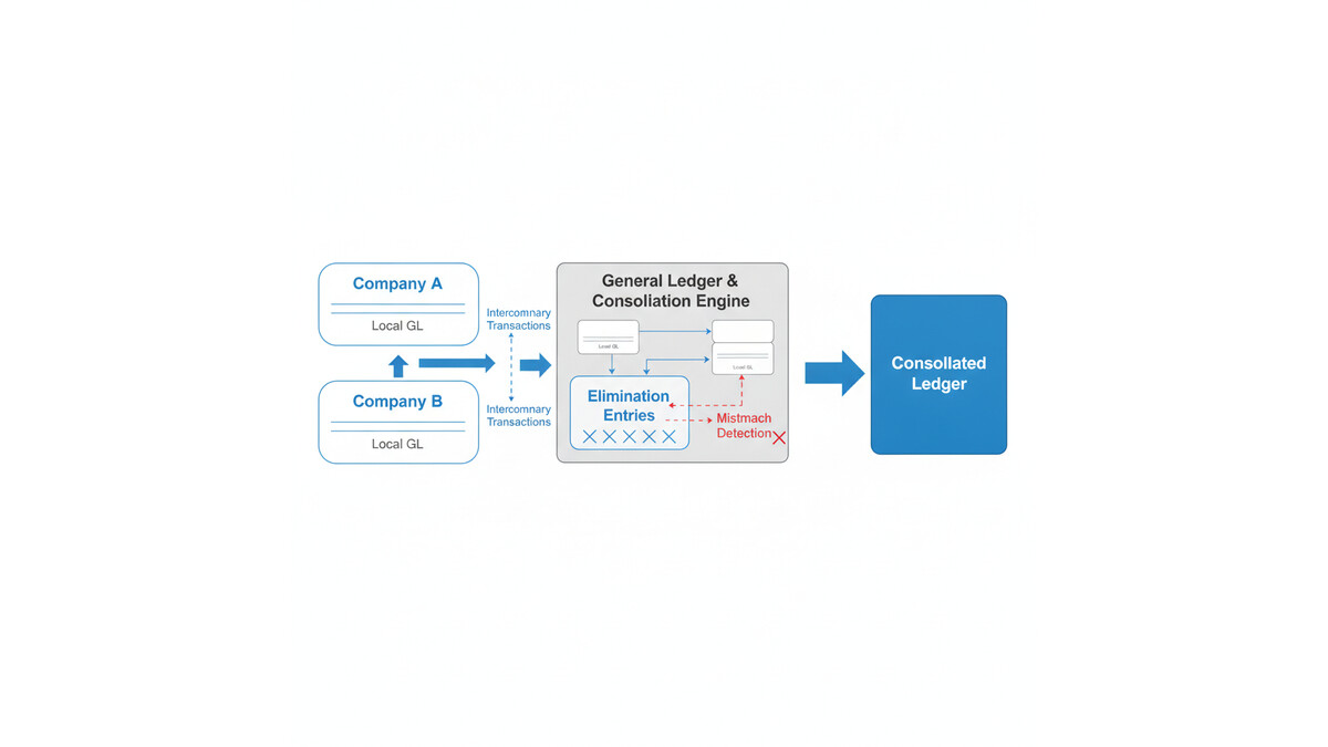
Dynamics 365 Finance treats intercompany transactions as a special case within the general ledger. When one legal entity (the originating company) records a transaction with another legal entity (the counterparty), both sides record the transaction independently. The originating company records the full transaction amount and an intercompany payable or receivable. The counterparty records the mirror transaction and an intercompany receivable or payable. These two sides are supposed to eliminate when you consolidate.

The elimination process is straightforward conceptually: find all intercompany balances, create offsetting entries to zero them out at the consolidation level, and produce a consolidated financial statement that shows only external transactions. In practice, Finance requires you to identify which accounts are intercompany balances, set up elimination rules, and ensure that the consolidation process knows how to match and eliminate transactions.

Where things diverge from this ideal is in the details of how intercompany transactions actually map to accounts. Finance assumes intercompany receivables and payables flow through specific account structures. If your chart of accounts doesn’t follow that structure, or if your intercompany transactions post to unexpected account combinations, the elimination logic can’t find matching pairs to eliminate.

Consolidated financial reporting process showing intercompany transaction flows and elimination logic

Why Elimination Entries Don’t Match Your Subledger

The root cause usually sits in one of three places: account mapping, transaction routing, or elimination rule configuration.

Account mapping issues: Intercompany receivables and payables need to map to specific accounts that the elimination process recognizes. If your chart of accounts assigns different accounts for intercompany activity than the elimination rules expect, transactions won’t match. For example, if you have intercompany sales recorded against one receivable account but intercompany service fees recorded against another, and your elimination rules only target the first account, service fee intercompany balances persist in the consolidated ledger.

Dimensional mismatch: Dimensions are where intercompany accounting often breaks down in practice. If your originating company records an intercompany transaction tagged with a specific cost center or business unit dimension, but the counterparty company records the mirror transaction without that same dimension combination, the two entries won’t find each other during elimination. The consolidation engine can’t match and eliminate transactions that have different dimension combinations, even if the account numbers and amounts are identical.

Timing and period mismatch: Intercompany transactions posted in one period in the originating company may not be received and matched in the counterparty company until the next period. If you try to run elimination at period-end before the counterparty company has received and recorded the transaction, the elimination process will create a temporary imbalance. This is especially common in month-end closes when one entity’s period ends before another’s, or when intercompany invoices are issued late in the month.

Control account vs. detail account confusion: Many implementations assign intercompany transactions to control accounts in the general ledger but then try to reconcile using subledger detail accounts. Finance’s elimination engine works at the general ledger level, not the subledger level. If the control account total is correct but the subledger detail account distribution doesn’t match what elimination expects, you’ll see reconciliation mismatches.

How to Diagnose the Problem

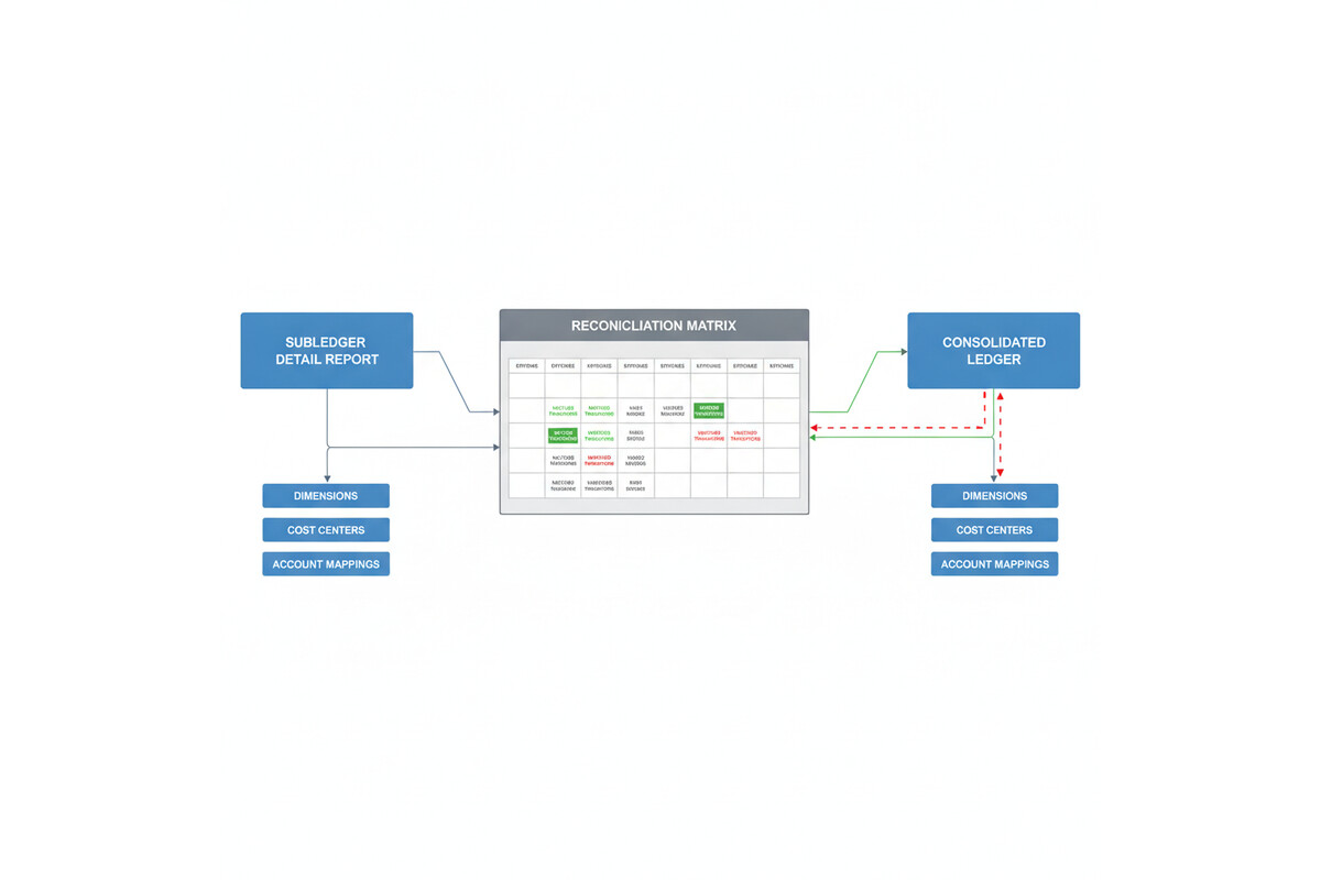
Start with a simple reconciliation: for each intercompany payable and receivable account, calculate the balance in the originating company’s general ledger, then calculate the mirror balance in the counterparty company’s general ledger. These two numbers should be equal and opposite. If they’re not, the problem is upstream of the elimination process.

If the balances match, the issue is in how the consolidation process is configured. Navigate to the consolidation elimination rules in Finance and verify that the account mappings and dimension rules are set up to match your actual posting. The elimination rules should specify which accounts contain intercompany balances, how they map between legal entities, and which dimension combinations are included in the elimination logic.

A common troubleshooting technique is to export the elimination entries that Finance generated, then manually reconcile them back to the intercompany transactions in your subledger. If the elimination entries don’t match specific subledger transactions, you’ve found the problem: either a transaction posted to an account the elimination rules don’t cover, or a dimension combination that doesn’t align between the two companies.

Intercompany reconciliation matrix showing matched and unmatched transaction entries

Designing Intercompany Accounting That Actually Eliminates

The cleanest approach is to standardize how intercompany transactions post across all legal entities. Define a consistent chart of accounts for intercompany receivables and payables, with the same account numbers used in every legal entity. If you use dimensions to tag transactions, establish a rule that intercompany transactions must be tagged with identical dimension combinations in both the originating and counterparty companies.

Consider whether you truly need dimensional detail on intercompany balances. Many implementations create dimensional complexity that adds no value to the intercompany reconciliation. If cost center assignment doesn’t affect how you manage intercompany payables, don’t require a cost center dimension on those transactions. Simpler account structures mean cleaner eliminations.

Set up a pre-consolidation reconciliation process in Finance. Before running elimination, generate a report of all intercompany balances, grouped by company pair, account, and dimension. Reconcile this to your subledger detail. If discrepancies appear, resolve them before you run the consolidation. This prevents the elimination engine from encountering unmatched transactions.

If you’re running multiple consolidation entities with nested parent-subsidiary relationships, test your elimination logic at each level. A common failure mode is that consolidation works correctly at the first level (subsidiary to intermediate parent) but breaks at the second level (intermediate parent to ultimate parent) because dimension combinations or account assignments drift as you go up the hierarchy.

When to Use External vs. Internal Elimination

Finance supports two elimination approaches: internal elimination (within Finance, using the consolidation module) and external elimination (in a separate consolidation tool or process). Internal elimination is simpler if your intercompany transactions follow a clean, standardized structure. External elimination is more flexible if your transactions are complex or your intercompany relationships don’t fit Finance’s default assumptions.

If you’ve been troubleshooting intercompany eliminations for months and the mismatches persist, it may be worth evaluating whether an external consolidation engine better serves your structure. Some organizations find that moving complex intercompany and consolidation logic to a dedicated consolidation tool reduces the burden on the Finance general ledger and makes the close process more transparent.

Preparation for Implementation

If you’re building an intercompany accounting structure from scratch, start by documenting your actual intercompany flow: which companies transact with each other, what types of transactions (sales, services, loans, expense allocations), and whether dimensional detail is needed on each type. Then design your chart of accounts and elimination rules to match that flow exactly.

Before you go live, run a full consolidation cycle with representative historical data. Create test transactions that cover every intercompany transaction type, post them in both the originating and counterparty companies, and run elimination. Verify that the elimination entries match the transactions you created, and that the consolidated ledger balances correctly. If you find mismatches at this point, you’re catching them before real transactions are in the system.

Assign one person ownership of the intercompany reconciliation and elimination process. That person should understand how the system is configured, have access to the elimination rules and the subledger detail, and be responsible for ensuring the process runs correctly every month. Intercompany accounting has a way of drifting if no one is explicitly in charge of keeping it clean.

Intercompany accounting is one of the places where small configuration oversights create large reconciliation problems. Taking time upfront to design and test your structure eliminates months of frustration during the close process.


Routeget Technologies: Our Finance & Operations consulting team helps enterprises design and implement intercompany accounting structures that consolidate cleanly and close on time, whether you’re building from scratch or fixing an existing implementation that’s struggling with elimination reconciliation.

#IntercompanyAccounting #Dynamics365Finance #FinanceImplementation #ConsolidatedReporting #ERPGovernance #AccountingAutomation #FinanceOperations #Dynamics365Implementation

Why Your Sales Teams Miss Account History: Building a Customer Data Foundation That Actually Works

Your sales rep is three weeks into a high-value deal. The prospect sends an email with a technical question about API integration. Your rep forwards it to the solutions architect, but there’s a gap: the solution architect doesn’t know that this same prospect raised the same concern in a customer service case six months ago, and the issue was already resolved. The rep and the architect spend two days re-solving a problem that was already closed. The deal slips by four weeks. The customer eventually buys, but at a lower margin because you spent double the resources.

This isn’t a technology failure. It’s a data foundation failure. Dynamics 365 Sales works beautifully when account history is available, connected, and accessible in real time. When it isn’t, your sales teams operate blind.

The Customer Data Foundation Problem

Dynamics 365 Sales is built for transparency. Every interaction, touchpoint, and detail about a customer should flow into a single, unified picture. In theory, your CRM contains everything: sales calls, email conversations, support cases, service interactions, contract history, purchase records, and even indirect interactions like website behavior. In practice, most organizations run multiple systems in parallel, and Dynamics 365 Sales sees only fragments.

A prospect visits your website. That behavior sits in your marketing automation tool. The same prospect opens a support ticket. That history lives in a separate service module, sometimes even a different Dynamics 365 instance. Your sales rep meets with the account team. The meeting notes go into email or OneNote, not into CRM. By the time your rep views the account record, they see a fractured picture: a contact history, some opportunities, maybe a few email messages, but no sense of the full customer journey.

The cost shows up in productivity loss, longer sales cycles, and missed upsell opportunities. More subtly, it shows up in deal risk: your sales teams make decisions based on incomplete information, leading to longer negotiations, missed risk signals, and post-sale surprises.

Why This Happens

Most organizations don’t lack a CRM. They lack a data platform that treats the customer as the central entity and routes all relevant data there automatically.

Building this requires three layers to work in concert. First, data integration: every system that touches a customer must have an automated bridge to Dynamics 365. Second, data normalization: when the same customer appears in different systems under slightly different names, identifiers, or attributes, they must be recognized as one entity before the data is merged. Third, data governance: your organization needs rules about data quality, freshness, ownership, and access, so that when sales teams see an account record, they trust what they’re seeing.

Most implementations skip or minimize one or more of these. Integration is expensive and complex, especially with legacy systems. Normalization requires understanding your data schema deeply, and many organizations have multiple schema variants across regions or business units. Governance is abstract and political; it’s hard to justify the investment before the problems surface.

The result: Dynamics 365 Sales is implemented, the basic data is loaded, and then the platform sits at a 40-50% adoption rate, with sales teams treating it as a record-keeping system rather than an operational tool.

Building the Right Foundation

A customer data platform implementation in Dynamics 365 Sales requires starting with a clear scope. Most organizations make the mistake of trying to integrate everything at once, which leads to scope creep, budget overruns, and delayed value. Instead, start by answering: which data sources touch the largest portion of your customer base, and which of those would have the highest impact on sales productivity or deal safety if that data were available in real time?

For many B2B organizations, the answer is clear: service ticket history, website engagement, and past contract terms. A sales rep should open an account and immediately know if there’s an open support ticket, whether the customer visited your website in the past week, and what the contract renewal date is. That’s table stakes. Everything else is an enhancement.

Start with those three sources. Integrate them into Dynamics 365, set up automated matching rules so that a customer in your support system is recognized as the same customer in your CRM (this is harder than it sounds), and implement a data governance rule that these three fields are always current, always trusted. Set a target: within 90 days, you want 90 percent of your active sales accounts to have historical data from at least two of these sources visible in Dynamics 365.

After 90 days, measure the impact. Did sales cycle length change? Did win rates move? Did customer acquisition cost shift? Did rep adoption of CRM increase? Don’t guess; measure it. If the foundation is working, the metrics should show improvement. If not, diagnose whether the issue is data quality, system design, or adoption, and fix the root cause before you expand.

Only after you’ve validated the value of the core foundation should you expand to other systems. That second wave might include marketing automation, accounting, or project management data. By then, you’ll have experience integrating systems, cleaning data, and managing adoption; the second and third integrations will move faster and face less internal resistance because the business already sees the return.

Implementation Considerations

Dynamics 365 Sales doesn’t provide a unified customer data platform out of the box. You’ll need to either build integration layers yourself or license a middleware platform to handle the data flow. Microsoft Dataverse, which underlies Dynamics 365, can handle the volume and complexity, but the plumbing to get data in and keeping it fresh is not trivial.

Cloud-based middleware platforms like MuleSoft, Tata Consultancy Services (TCS) iPaaS, or native solutions like Azure Data Factory can automate the flow from source systems to Dataverse. The choice depends on your technical depth, the number of source systems, and your tolerance for managed services versus internal ownership. Budget-conscious organizations often underestimate the effort here; real-world integration projects are 60-70 percent data cleaning and schema mapping, not configuration.

Data governance is the second underestimated piece. Before you integrate a data source, your organization needs to decide: who owns this data? What’s the acceptable latency? If data in the source system changes, how quickly should Dynamics 365 reflect that change? What’s the fall-back plan if the integration breaks? Who monitors it? These questions are boring, but organizations that skip them end up in situations where sales reps stop trusting the data because updates are erratic, or where the system breaks and no one notices for weeks.

Adopt an incremental approach. Start with one source system, prove value, expand carefully, and measure at each step. That’s the path to a customer data foundation that actually works.

The Competitive Advantage

When your sales teams have a complete, current picture of each account, everything changes. Your reps spend less time gathering context and more time strategizing. Your AEs shorten sales cycles because they understand account history and can speak credibly about prior interactions. Your customer success teams have better handoff information, leading to higher retention. Your account teams spot upsell opportunities they would otherwise miss because they see the full engagement history.

In competitive deals, this advantage compounds. If your sales rep knows that a competitor pitched to the same prospect three months ago but was rejected over a specific feature concern, and your company has since shipped that feature, your rep can lead with that insight. The prospect feels heard and known. That’s the difference between a deal that is hard-won and a deal that moves smoothly.

The first step is admitting that your current CRM isn’t showing you everything you need to see. The second is committing to build the data foundation that makes that visibility real. Start small, measure honestly, and build from there. Your sales teams and your pipeline will thank you.


About Routeget Technologies: Routeget helps enterprise organizations design and implement customer data platforms on Dynamics 365. If your sales teams are working blind, we can help you build the foundation to fix it.

#DynamicsCustomerEngagement #CustomerDataPlatform #SalesProductivity #Dynamics365CRM #SalesEnablement #DataIntegration #CustomerInsights #SalesStrategy

Dataverse Calculated Columns and Rollups: When Summary Data Becomes a Bottleneck

Most Dynamics 365 implementations contain at least one field that should not exist. It is usually a number that sums values from child records, or a formula that derives from related data. The reason it exists is always the same: someone wanted real-time access to that information from a parent record, without running a report or opening a separate list.

Dataverse calculated columns and rollup columns promise to solve this problem. Calculated columns apply a formula to one or more fields on the current record, showing the result live without code. Rollup columns sum, count, average, or find min/max values from related records, showing that aggregation on the parent record. Both sound straightforward in a demo. Both become serious performance liabilities in production when misapplied.

The problem is not that calculated columns or rollups are poorly designed. The problem is that their flexibility and ease of configuration make it tempting to create them for every question a user asks, and because Dataverse computes these columns synchronously during record operations, each one you add delays every operation touching that record or its related data. At scale, calculated columns and rollups can turn a fast, responsive system into one where simple form loads lag and mass operations hang.

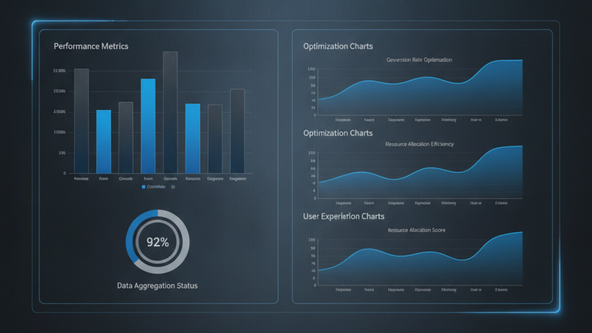
Performance metrics dashboard for database optimization

How Dataverse Calculated Columns and Rollups Actually Work

Calculated columns in Dataverse run when a record is created, updated, or retrieved. Unlike plugin code you can optimize or disable, calculated columns execute on every interaction. If you define a calculated column that divides a budget by a count of child records, that division happens every time anyone loads the form, every time a Power Automate flow retrieves that record, and every time an integration fetches the data via the API.

Rollup columns add another layer of complexity. A rollup does not just read data from related records; it must traverse a relationship, evaluate a condition on each related record, and then compute the aggregation. If you create a rollup that counts all incomplete tasks related to an account, Dataverse must walk through every task record linked to that account, check each one’s status, and return the count. On an account with 50,000 tasks, this query can take seconds.

Both calculated columns and rollups are recomputed on a schedule. Dataverse does not compute them in real-time on demand; instead, the system recalculates them asynchronously in batch jobs. This means that displayed values may not always reflect the absolute latest state of the source data. For a dashboard or a report, this lag is usually acceptable. For a workflow that needs to make a decision based on that value, the delay can cause logic to fail or bypass critical checks.

When Calculated Columns and Rollups Become Problems

Performance issues with calculated columns and rollups typically emerge at one of three trigger points.

First is load time. A form containing multiple calculated columns or rollups can take noticeably longer to render, especially on mobile or slower connections. Users perceive this as a slow or unresponsive system. The impact scales with the number of columns; a form with 2 or 3 calculated fields performs fine, but one with 10 or more can lag visibly.

Second is mass operations. Bulk operations such as Power Automate loops that create or update thousands of records will execute more slowly if those records contain calculated columns or rollups. Each record operation pays the calculation cost, so a loop that would normally complete in 30 seconds might take 3 minutes. Workflows that timeout during scheduled jobs often have calculated columns as a hidden root cause.

Third is query performance. Reports or Power BI dashboards that query many records will hit slowdowns if the records contain expensive calculated columns or rollups. The calculation must complete before the record is returned, so querying 10,000 records with heavyweight calculations forces Dataverse to compute all 10,000 calculations before the query finishes.

A fourth, more subtle issue is the logical inconsistency created by asynchronous recalculation. If a workflow reads a rollup column value, performs business logic based on that value, and then the rollup recalculates a moment later and changes, the workflow has acted on stale data. This can create gaps in audit trails or cause business logic to diverge from the actual state the user sees.

Detecting Bottlenecks

Before optimizing, you need to know if calculated columns or rollups are actually the problem. A few diagnostic approaches work.

Check the Dataverse environment’s performance reports. Look for slow-running queries or forms that take longer than expected. If a form with calculated columns loads in three seconds and the same form without them loads in one second, the columns are adding two seconds of latency. Similarly, check Power Automate run histories for timeouts or slow execution in flows that work with records containing rollups.

Enable Plugin Trace Log (under Settings in your Dynamics environment) and examine traces for records being retrieved with calculated columns. Look at the duration of retrieve operations; if simple record retrievals are taking longer than 500 milliseconds, calculated or rollup columns are a likely culprit.

Query the Dataverse API directly with and without calculated columns in the result set. Use select parameters to request only the columns you need. If adding a calculated column to the query selection significantly increases response time, you have confirmed the issue.

Database schema showing parent-child record relationships and calculation flows

Alternatives to Calculated Columns and Rollups

If you have identified a bottleneck, you have several options. The best choice depends on your specific scenario.

Use plugins or Power Automate to calculate on demand. Instead of computing the value every time a record is retrieved, calculate and store it only when necessary. A plugin triggered on form load can calculate a summary and display it in a banner, showing fresh data without impacting record retrieval. A Power Automate cloud flow can run on a schedule to update rollup values once per hour or once per day, depending on your tolerance for staleness. This approach keeps the permanent record lean.

Move calculations to the reporting layer. Power BI does not care if a column is calculated in Dataverse or computed in the dataset; the result looks the same to an end user. Create a calculated column in a Power BI dataset instead of in Dataverse, and use that column only for dashboards and reports. Forms and integrations get the base data without calculation overhead.

Use views and roll-up jobs sparingly. If you do use rollups, create them for only the most critical summaries. A single rollup that counts open orders on an account is reasonable; four rollups that count open orders, sum order amounts, calculate average order value, and find the date of the latest order should be four separate on-demand calculations in Power Automate or a custom plugin.

Denormalize selectively. For high-cardinality relationships (an account with tens of thousands of related records), consider storing pre-calculated values in a separate summary table updated by a scheduled batch process, rather than relying on Dataverse to calculate them live. This trades a small amount of design complexity for significant performance gains.

Production-Ready Patterns

In practice, high-performing Dataverse implementations keep calculated and rollup columns minimal. A good rule of thumb: if a column is not displayed on a form or used in a critical workflow decision, it should not exist as a calculated or rollup column.

When you do create them, profile the specific form or report where they appear. Measure load time before and after; if latency increases by more than 200 milliseconds per column, investigate alternatives. For rollups, test with realistic data volumes; a rollup that works fine with 100 related records may not work at all with 10,000.

Document which forms, reports, and integrations depend on each calculated or rollup column. This becomes essential when troubleshooting slow operations; knowing that a dashboard uses a particular rollup helps you understand why it is not refreshing quickly.

Finally, review calculated and rollup columns every few months. As your implementation matures and data volumes grow, columns that performed acceptably in early stages may become bottlenecks. Removing a column that no longer serves a critical business purpose often has an immediate, measurable impact on overall system responsiveness.

Calculated columns and rollups are powerful tools when used deliberately. They become performance anchors when used casually. The teams that manage Dataverse best treat them not as convenience features, but as performance decisions that must be justified by real business need and validated through testing at production scale.


#DataversePerformance #CalculatedColumns #RollupOptimization #DataverseTuning #Dynamics365Performance #CloudArchitecture #DataverseArchitecture #SystemPerformance

Business Central for Growing Manufacturers: Why Your ERP Doesn’t Need to Cost $500K/Year

“

Why Legacy ERP Cost So Much

\n\n

On-premises ERP systems impose costs at three points that most CFOs misunderstand until they are deep into a migration project. First, there is the initial software license cost, which for large suites often runs between fifty and one hundred fifty thousand dollars upfront, plus annual maintenance fees that compound every year. Second, and more significant, is implementation cost. A team of five consultants embedded for twelve to eighteen months at typical rates adds two hundred to three hundred fifty thousand dollars, sometimes more.

\n\n

Third, and often overlooked, is the ongoing operational cost. On-premises systems require dedicated infrastructure, whether owned or leased. Database administration, system patching, security monitoring, and backup management all fall to your IT team. A medium-sized manufacturer typically allocates at least one full-time employee, sometimes more, to keep the system running, preventing outages, and managing infrastructure growth as data volume increases.

\n\n

The perpetual license model also creates a perverse incentive to extend the useful life of outdated systems. Once you have spent half a million dollars, retiring the system in five years feels wasteful. So manufacturers keep systems in production for ten, twelve, or fifteen years, long past the point where modern capabilities could improve operations. Meanwhile, the system becomes increasingly fragile. Every upgrade risks instability. Reporting requires manual steps because the database schema no longer accommodates new business logic. Integration to modern tools like Microsoft Teams or Power BI requires custom bridges that consume engineer time.

\n\n

Business Central breaks this cost structure at every stage.

\n\n

Business Central’s Cost Foundation

\n\n

Business Central runs on the cloud, which means no infrastructure cost for you to manage. Microsoft owns and maintains the servers, databases, backup systems, and security infrastructure. Your finance and operations team still has full access to configuration, reporting, and business logic customization. But the system administration overhead shifts to Microsoft.

\n\n

The licensing model reflects this shift. A Business Central user license currently runs between $50 and $140 per month depending on the tier, with no perpetual license, no infrastructure fee, and no hidden per-transaction cost. A typical mid-market manufacturer with 100 to 150 active users in finance, operations, supply chain, and manufacturing would spend $60,000 to $250,000 annually on user licenses. Compare that to the upfront costs of enterprise ERP, and the difference is immediately clear: Business Central’s annual cost can be lower than the implementation cost of older systems.

\n\n

The implementation timeline for Business Central also compresses dramatically. A well-scoped Business Central implementation for a manufacturer typically completes in four to eight months, not eighteen. Core financial management, inventory control, and basic manufacturing production scheduling can be operational within that timeframe. A smaller implementation might need only four weeks to three months. That speed exists because the system arrives with reasonable defaults for standard business processes. You are not building a system from scratch. You are configuring a system that already understands accounts payable, inventory valuation, and bill-of-materials logic because that is what every manufacturer needs.

\n\n

A typical Business Central implementation for a mid-market manufacturer might engage two to four consultants for four to six months, which translates to $80,000 to $240,000 in consulting services, depending on regional rates and the extent of custom reporting or integration needs. For comparison, that is in line with the annual ongoing cost of maintaining a legacy system with dedicated IT staff, and you are paying it once, not every year indefinitely.

\n\n

What Business Central Gives You

\n\n

The faster implementation and lower ongoing cost matter only if the system delivers the capabilities a manufacturer actually needs. Business Central includes standard functionality for the core business processes that define manufacturing operations.

\n\n

Financial management in Business Central covers general ledger accounting, accounts payable, and accounts receivable without requiring custom configuration. Multi-company consolidation is built in, which matters to organizations with multiple manufacturing facilities or regional operating entities. Tax calculation integrates with native modules, and the platform supports multiple currencies and statutory reporting requirements across different countries, important for manufacturers with any international operations or sales.

\n\n

Inventory management handles lot tracing, serial number tracking, and expiration date management, all capabilities required by regulated manufacturers. The system supports standard costing, moving average, FIFO, and other valuation methods. Cycle counting, physical inventory reconciliation, and intercompany inventory transfer all work without custom code.

\n\n

Production scheduling and shop floor management in Business Central use visual production scheduling, work center definitions, and routing setup. The system calculates material requirements based on bill-of-materials structures and translates production schedules into purchase orders for raw materials. For job shops or custom manufacturers, production orders can be linked to sales orders, so each job’s profitability is tracked separately.

\n\n

Purchasing and supplier management allow you to define purchase agreements, track supplier performance, and manage invoice matching. Multi-level approval workflows prevent unauthorized spending.

\n\n

What Business Central does not include, and what some larger manufacturers require, is distributed manufacturing across a complex supply network, advanced demand planning with statistical forecasting, or deeply customized shop floor control logic. If your manufacturing operation is relatively standard, if you make primarily to stock or engineer to order without extreme complexity, if you operate one or two facilities, Business Central will fit. If your operation requires the scale of Dynamics 365 Supply Chain Management to manage global supply networks or highly complex planning logic, Business Central is not the answer.

\n\n

The Real Cost Comparison

\n\n

A manufacturing organization with 150 active users, a single factory, and standard ERP requirements might spend:

\n\n

With Business Central: $180,000 annually on user licenses (150 users times $120 per month times 12 months divided by 12), plus $150,000 in implementation consulting over four months, for a total first-year cost of $330,000. Year two cost drops to $180,000 annually since implementation is complete.

\n\n

With enterprise ERP on premises: $150,000 in perpetual software licenses, $300,000 in implementation consulting over 18 months, $80,000 annually for database administration and infrastructure management, and miscellaneous annual maintenance and upgrades. Year one cost is $430,000; every year after is $230,000 indefinitely.

\n\n

By year three, the organization using Business Central has spent $690,000 total. The organization using enterprise ERP has spent over $890,000 and will spend $230,000 every year going forward. The payback period for migrating to Business Central, if that option exists, is typically between three and four years for a mid-sized manufacturer.

\n\n

That financial calculation assumes the enterprise system remains operational without major problems, major upgrades, or unexpected infrastructure failures, which is not always realistic for fifteen-year-old systems.

\n\n

Beyond the Initial Implementation

\n\n

Business Central also integrates directly with Microsoft 365 and Power Platform tools, which many manufacturing organizations already use for email, collaboration, and office productivity. Accounting data can be analyzed in Power BI without additional ETL or data warehouse setup. Office integration means finance teams can work with Excel, Word, and Teams directly with ERP data without exporting and re-importing.

\n\n

If a manufacturer later needs to scale, Business Central can coexist with Dynamics 365 Supply Chain Management or Finance and Operations for specific functions. A common pattern is to run Business Central for accounting and operations, then layer Supply Chain Management on top if manufacturing complexity or global supply network needs increase later. That staged approach spreads capital expenditure over time and allows you to prove ROI before investing in enterprise licensing.

\n\n

When Business Central Is Not the Right Answer

\n\n

For extremely high-volume manufacturers, organizations with complex engineering-to-order processes, or manufacturers operating hundreds of facilities across different regulatory jurisdictions, Business Central’s simpler data model and configuration limits may become constraints. Dynamics 365 Supply Chain Management and Finance and Operations exist for those scenarios. But those scenarios represent a small fraction of manufacturers.

\n\n

For the mid-market manufacturer currently on an outdated system, believing that only enterprise ERP justifies modernization, the real question is not whether Business Central is capable enough. It almost certainly is. The question is whether staying on legacy infrastructure is really more cost-effective than moving forward. For most manufacturers, the answer is no.

\n\n


\n\n

#BusinessCentralERP #ManufacturingERP #Dynamics365CloudERP #SMBERPSolutions #ManufacturingCostReduction #CloudAccountingSystems #Dynamics365BusinessCentral #ERPImplementation

\n”