
Reducing Supply Chain Visibility Gaps in Dynamics 365: How Planning Drives Just-In-Time Operations Without Safety Stock Bloat

Reducing Supply Chain Visibility Gaps in Dynamics 365: How Planning Drives Just-In-Time Operations Without Safety Stock Bloat

Supply chain directors face a familiar and frustrating trade-off: either maintain substantial safety stock buffers to absorb demand and supply variability, tying up millions in working capital, or run lean inventories and endure constant firefighting, expedited shipments, and overtime labor. Most organizations choose poorly on this calculation, erring toward excess stock precisely when their working capital metrics need relief.

The core problem is visibility. Even with ERP systems in place, most supply chains operate on a foundation of disconnected demand signals, manual forecast adjustments, and reactive purchasing driven by stockout fear rather than data. Sales makes a forecast in their system; supply chain plans in another silo; suppliers react after the fact. By the time everyone sees the same picture, decisions have already locked in expensive safety stock or created a panic order.

Dynamics 365 Supply Chain Management (SCM) addresses this differently. When integrated with realistic demand planning, supplier integration, and real-time inventory visibility, D365 SCM shifts the equation: your safety stock levels can drop 15 to 30 percent while simultaneously reducing expedites and manufacturing overtime, because your organization finally has the visibility and planning automation to match supply to actual demand rather than worst-case fear.

The Real Cost of Inventory Misalignment

Consider a mid-market manufacturer managing 5,000 SKUs across four distribution centers and three contract manufacturing partners. Without strong demand-supply integration, this organization typically carries 45 to 60 days of safety stock across the network to absorb unexpected demand spikes and supplier variability. At an average holding cost of 25 percent annually (which includes warehouse space, insurance, shrinkage, and obsolescence risk), this represents roughly $8 to $10 million in working capital entirely dedicated to “just in case.”

Worse, the safety stock isn’t actually preventing problems. When demand truly spikes, the organization still expedites shipments from suppliers (at 15 to 30 percent premiums) and runs overtime in manufacturing. When demand falls short, inventory ages and eventually must be written down. Safety stock is expensive insurance that doesn’t actually cover the risk. A typical mid-market organization writes off 2 to 5 percent of inventory annually due to obsolescence, aging, or damage—often thousands of dollars lost to products that were supposed to be protective buffers but instead became ballast.

The real driver of this inefficiency is simple: supply chain decisions are made on incomplete information. Demand planning happens separately from supply planning. Sales forecasts sit in one system; procurement works from outdated demand signals; manufacturing schedules are locked in before demand visibility improves. By the time data flows between systems, it’s stale, and decisions compound the problem.

Integrated Demand and Supply Planning in D365

Dynamics 365 SCM solves this through three integrated mechanisms: centralized demand sensing, collaborative planning, and automated supply network optimization.

Demand sensing in D365 aggregates inputs from sales forecasting, point-of-sale data (where available), and forward-looking demand signals such as customer orders and promotional calendars. Rather than treating the forecast as a one-time input, D365 continuously updates it as new orders arrive and actual sales data flows in. A promotion forecasted to drive 20 percent demand lift is immediately visible across supply chain planning the moment it’s confirmed in the sales system. No waiting for month-end reconciliation.

Collaborative planning connects procurement, manufacturing, and logistics into a shared planning view. When demand updates, D365 recalculates required inventory levels across the supply network in near-real time. If demand in the Southwest region is tracking 10 percent higher than forecast, D365 recommends either accelerating shipments from your closest manufacturing location or increasing safety stock slightly in that region specifically, not across your entire network. The algorithm trades off transportation costs, carrying costs, and service level targets to recommend the most economical move.

Supplier integration completes the loop. When your procurement team plans a large purchase order, D365 can directly feed visibility to suppliers capable of receiving such data. Instead of planning with a standard six-week lead time assumption, you see actual supplier capacity and can negotiate shorter lead times for critical components. Conversely, when your forecast drops, suppliers see that immediately, reducing the bullwhip effect where supply chain players over-order to protect inventory because they lack confidence in their demand signal.

Working Capital Impact and Operational Efficiency Gains

Organizations that implement this integrated approach typically reduce safety stock levels by 15 to 30 percent within the first 12 months. For a $500 million revenue manufacturer with $50 million in inventory, this translates directly to $7.5 million to $15 million in freed working capital. For a CFO watching cash conversion cycles, this is material: a 20 percent inventory reduction on a $50 million balance sheet is equivalent to a sales increase of 15 to 20 percent in terms of working capital impact, but without the cost of actually growing revenue.

Equally important, operational friction drops. Manufacturing runs smoother because production schedules reflect actual demand rather than buffer stock concerns. Procurement teams spend less time expediting and more time managing supplier performance and cost reduction. Distribution centers reduce reverse logistics (product returns and aging stock write-downs) because inventory is right-sized to actual demand.

The expedite cost reduction alone often funds the initiative. If your organization historically expedites $2 to $3 million worth of shipments annually (a typical figure for mid-market supply chains), reducing expedites by even 40 percent generates $800K to $1.2M in annual savings. Better visibility and planning make that reduction achievable without service level risk. Most organizations report that expedite costs drop by 50 to 60 percent once demand visibility improves, since the root cause of expedites isn’t usually a sudden unpredictable spike but rather the organization’s own poor forecast accuracy creating artificial scarcity.

Critical Success Factors

Realizing these benefits requires discipline in three areas. First, demand forecasting accuracy must improve materially. D365’s planning engine is only as good as the input. If sales continues to provide wildly inaccurate forecasts, safety stock levels stay high. Many organizations find they need to implement a more rigorous sales and operations planning (S&OP) process, with monthly reconciliation of sales forecast vs. actual and bias correction. This is organizational work, not software work. Plan to invest 4 to 6 weeks in S&OP process design and 2 to 3 months of monthly iterations before forecast accuracy stabilizes.

Second, data quality across the supply network must be reliable. Inventory balances, lead times, supplier performance, and demand signals must flow into D365 with high fidelity. If your manufacturing system doesn’t accurately report on-hand balances or your POS data arrives three days late, planning decisions sit on a weak foundation. Most organizations need 2 to 4 months of data cleanup and integration work before planning accuracy truly improves. Expect to find that 5 to 15 percent of your current inventory doesn’t match physical counts, and allocate resources to reconciliation.

Third, safety stock policy must shift from “assume worst case” to “plan with confidence.” This is cultural. Your finance and operations leaders need to agree on a target service level (usually 95 to 99 percent for most products) and trust that the planning engine, with better visibility, can hit it with lower safety stock. Organizations that resist this mindset end up keeping old safety stock levels even after visibility improves, negating the working capital benefit entirely. Executive alignment on acceptable service level targets is often the difference between success and stalled projects.

The Path Forward

Supply chain directors evaluating D365 SCM should focus the business case on working capital relief and operational efficiency rather than on a vague promise of “better planning.” Quantify your current safety stock, your annual expedite costs, and your inventory write-down rate. Model a 20 percent improvement in each as a conservative scenario and commit to the changes in forecast discipline, data quality, and planning policy that make it real. Over 18 months, the working capital freed up typically far exceeds the implementation cost.

The competitive advantage is no longer in having the most stock; it’s in having the most accurate demand visibility and the discipline to act on it. Dynamics 365 SCM provides the visibility and automation. The execution depends on your organization’s commitment to better planning discipline and the courage to trust data over pessimism.

Consolidating Multi-Subsidiary Financial Operations in Business Central: How SMBs Achieve Real-Time Visibility and Faster Close Cycles

Introduction

Most finance leaders managing multi-subsidiary organizations face a recurring problem: subsidiary teams submit monthly close packages on different schedules, using different chart-of-account structures, reporting in different currencies, and operating on separate systems. The consolidation process becomes a spreadsheet orchestration nightmare, with Excel feeds from three or four subsidiaries arriving late, requiring manual reconciliation and multiple rounds of revision before final consolidated financials can be reported. In a mid-sized organization with five to ten subsidiaries, this process routinely stretches beyond the 15th of the month, delaying board reporting and decision-making.

Business Central, when properly structured, eliminates this friction. By deploying a unified chart-of-accounts framework across subsidiaries, enabling real-time data synchronization through Power Platform connectors, and automating currency conversion and elimination entries, organizations can close the books consolidated within 2-3 days rather than 10-15 days.

The Current State: Manual Consolidation and Its Costs

In a typical pre-Business Central environment, each subsidiary maintains its own legacy ERP or general ledger. Finance downloads trial balances from each system, translates accounts to a common chart-of-accounts structure using lookup tables in Excel, applies currency conversion rates for foreign subsidiaries, and begins manual data entry. Visibility into real-time subsidiary balances disappears because consolidation always lags the close date. Finance staff spend 20-30 percent of month-end on consolidation alone, junior accountants spend evenings cross-checking submissions, and the organization misses opportunities to identify profitability issues in real time.

Why Unified Chart-of-Accounts Matters

The first decision when deploying Business Central across subsidiaries is structural: will each subsidiary have its own independent Business Central company, or will they all report into a single Business Central tenant with a unified chart-of-accounts?

In a unified structure, each subsidiary operates a separate Business Central company, but they all map transactions to an identical chart-of-accounts structure. A revenue account numbered 4100 in the parent is also 4100 in every subsidiary. The parent company can pull consolidated trial balances directly from the Business Central database in seconds, rather than waiting for manual submissions and mapping.

The tradeoff is upfront effort: establishing a truly unified chart-of-accounts requires that parent finance leadership and subsidiary teams align on account naming, numbering, cost-center structure, and dimension tags before implementation, typically taking 4-8 weeks. Once it is in place, month-end reporting becomes a database query rather than a manual assembly line.

Real-Time Data Synchronization

Once chart-of-accounts alignment is in place, real-time data availability transforms the consolidation process. Rather than waiting for month-end submissions, a unified Business Central instance can pull live subsidiary data continuously using Power Automate flows. Each subsidiary’s Business Central company validates close nightly; at 8pm, a Power Automate flow pulls the latest trial balance, standardizes it to the parent’s chart-of-accounts structure, and stores it in a Dataverse table that acts as the parent company’s “live consolidation view.” By morning, the CFO can log in to Power BI and see exactly where each subsidiary stands, in real-time.

Currency conversion happens within this flow automatically, using centrally maintained Exchange Rate tables. The parent company’s accounting system knows, in real-time, that Subsidiary A operating in Euros has closed 15 million EUR in operating expenses, which converts to 16.2 million USD at current rates. No spreadsheet. No manual lookup. This continuous visibility enables finance leaders to spot issues early in the month, such as an unexpected variance in one subsidiary’s cost structure, rather than discovering them during the formal consolidation window.

Handling Currency Conversion and Intercompany Eliminations

Currency conversion in a multi-subsidiary environment often looks simple until intercompany transactions across multiple currencies create rounding differences that cascade through consolidation. Business Central handles this through exchange rate tables set to month-end rates, with consolidation posting routines automatically applying those rates to subsidiary balances during the consolidation step.

Intercompany eliminations require more careful setup. A common scenario: Subsidiary A (USD) buys inventory from Subsidiary B (EUR). From Subsidiary A’s perspective, this is a cost and a payable. From Subsidiary B’s perspective, it is revenue. From the consolidated perspective, both net to zero. The right approach is to define intercompany relationships in Business Central and use automated elimination routines that match intercompany entries, convert to a common currency, and eliminate both sides through a Power Automate flow or custom extension.

Implementing in Phases

Deploying Business Central consolidation across 3-10 subsidiaries typically requires four phases:

Phase 1: Foundation (Weeks 1-6): Establish unified chart-of-accounts across parent and 1-2 pilot subsidiaries. Conduct workshops to align account structure, cost-center mapping, and close procedures. Configure Business Central companies and migrate 12-24 months of historical GL balances. Run parallel close cycles for 1-2 months before cutover.

Phase 2: Automation (Weeks 7-12): Build Power Automate flows to pull trial balances from subsidiary companies, apply currency conversion, and populate consolidation staging tables. Create Power BI dashboards showing consolidated trial balance updated daily. Define and code intercompany elimination rules as Power Automate flows. Run consolidated close cycle entirely within Business Central for 2-3 months.

Phase 3: Rollout (Weeks 13+): Deploy Business Central to remaining subsidiaries one or two per month, following the same phased approach. As each subsidiary goes live, add its data to the consolidation automation.

Phase 4: Continuous Improvement (Ongoing): Expand Power BI dashboards to include subsidiary-level profitability, cash flow, and working capital metrics. Use this data to drive operational decisions at the subsidiary level.

Real-World Impact

Organizations implementing Business Central consolidation across 3-5 subsidiaries typically report substantial outcomes within 12 months. Consolidation close time drops from 10-15 days to 3-5 days, enabling earlier board reporting and faster decision-making. Finance staff freed from consolidation mechanics gain meaningful capacity to focus on analysis, variance investigation, and forecasting. Real-time visibility to subsidiary financial data, accessible through Power BI dashboards, supports faster identification of profitability issues, cash flow concerns, or operational anomalies that warrant investigation. Manual transcription and rounding errors inherent in spreadsheet-based consolidation disappear entirely, improving audit readiness and reducing the variance investigation cycles that typically consume several days post-close. Adding a new subsidiary becomes operationally straightforward—you deploy Business Central, configure the new subsidiary to the unified chart-of-accounts, and add it to the consolidation automation, with no material increase in consolidation time or complexity.

Key Considerations

Unified consolidation requires meaningful upfront investment in chart-of-accounts alignment. If subsidiaries actively transact with each other, intercompany elimination entries require monthly review and become a significant consolidation component. Many subsidiaries need local statutory reporting separate from consolidated financials, requiring separate reporting structures. Most importantly, data quality discipline is foundational; automation amplifies poor GL posting practices. Invest early in GL validation rules within Business Central at the subsidiary level.

Conclusion

Consolidating multi-subsidiary financial operations in Business Central is a practical path to faster, more accurate month-end close and real-time financial visibility. It requires upfront investment in chart-of-accounts alignment and automation setup, but the payoff is measurable: consolidated financials in 2-3 days rather than 10-15 days, finance staff freed to focus on analysis rather than mechanics, and subsidiary-level visibility supporting operational decision-making.

For mid-market organizations operating with 3-10 subsidiaries, this capability is well within reach and delivers substantial benefits to finance operations and organizational agility.


About Routeget Technologies

Routeget Technologies specializes in deploying Dynamics 365 and Business Central across multi-entity organizations, with deep expertise in consolidation automation, global payroll integration, and multi-currency operations. If your organization is evaluating Business Central consolidation, reach out to discuss your specific situation and objectives.


#ConsolidationAutomation #BusinessCentralFinance #MultiEntityERP #FinanceTransformation #DynamicsERP #SMBAccounting #RealTimeFinancials #ERPImplementation #FinanceOps #MidMarketERP

Managing Dataverse Capacity and Archival: Cost Optimization and Compliance for Growing Dynamics 365 Deployments

Managing Dataverse Capacity and Archival: Cost Optimization and Compliance for Growing Dynamics 365 Deployments

By the time most finance and operations teams reach their second or third year running Dynamics 365, they face a familiar problem: storage costs climb faster than anticipated, and the expense of adding capacity becomes a line item that catches CFO attention.

Dataverse capacity management is not optional complexity. It is operational and financial necessity. The decision about how to handle growing data volumes determines whether your Dynamics 365 environment scales affordably over the next five years, or whether you find yourself funding expensive capacity add-ons every year while your system performance degrades and your operational data becomes less accessible for decision-making.

The good news is that Dynamics 365 now provides a structured path to address this problem. Rather than simply buying more storage, organizations can implement a data lifecycle strategy that reduces live database footprint by 40 to 50 percent while keeping historical data accessible for audit, compliance, and analytical purposes.

The Real Cost of Dataverse Storage Growth

Dataverse capacity does not cost a fixed amount. Dynamics 365 operates under a tiered licensing model where storage overages trigger additional charges per gigabyte. Organizations with 100 GB of storage consume licensing differently than those with 500 GB. The financial pressure accelerates as deployments mature because data accumulates across all functional areas simultaneously: general ledger and subledger transactions grow at transaction volume rates, inventory movements accumulate, sales orders and purchase orders multiply, and attachments expand without structural limits.

The attachment problem alone deserves specific attention. In most live Dynamics 365 environments, attachments and unstructured documents consume the majority of file storage. A single large document attached to a purchase order, added across thousands of orders over multiple years, creates unexpected storage bloat. Because Dataverse charges capacity fees on total database size, every attachment carries an ongoing cost, whether the underlying transaction remains relevant for daily operations or not.

This is why many organizations discover, mid-year, that their projected storage consumption was low by a factor of 2 or 3. The discovery comes when the platform sends a near-capacity warning, forcing a decision between purchasing additional storage immediately or undertaking a remediation project that may take weeks.

Archival: A Strategic Three-Layer Approach

Microsoft’s archival and long-term retention framework provides a structured alternative to unlimited growth. Rather than treating all data as equally important to the live system, the approach moves data through three operational tiers based on access patterns and compliance requirements.

The first tier remains live transaction data: current orders, active customers, outstanding payables, inventory on hand, general ledger accounts in the current and prior fiscal year. This data stays in the primary Dataverse tables and participates in real-time queries, reports, and daily operational workflows. It receives the full performance and availability guarantees of the live system.

The second tier is history tables. Records meeting archival criteria move to specialized history tables within Finance and Operations, where they remain queryable but occupy approximately 30 percent less storage than live tables because indexes are minimized and the data is marked read-only. Users can still access historical transactions through inquiry pages and can restore specific records if needed, but the system no longer treats them as active for daily operations.

The third tier is long-term retention in Dataverse. Records in Dataverse long-term retention tables, marked with a “-Retained” suffix, are read-only and consume the lowest storage footprint of all three tiers. They remain accessible for compliance reporting, historical analysis, and audit trails, but they do not participate in operational workflows. For organizations managing decades of transaction history, this tier can be configured to store data that must be retained for regulatory or audit purposes but never accessed in operational workflows.

Microsoft’s testing has shown that moving data from live Dataverse tables to long-term retention reduces capacity consumption by approximately 50 percent, though actual savings depend on data composition and table structure.

Implementation Strategy: Three Decisions

Before archival can be deployed, organizations need to make three distinct decisions.

First, which tables should be archived. Not every table is a candidate. Finance and Operations currently supports archival for general ledger transactions, tax transactions, sales orders, inventory movements, and related journals in supply chain and commerce. Custom tables can be included if they follow established data structures, but archival is not available for all tables in your deployment. Prioritize high-volume transactional tables where historical data is unlikely to be modified.

Second, what archival frequency makes sense. Many organizations implement annual archival, moving records older than 18 or 24 months to history tables once per year. Others implement rolling monthly archival, moving older cohorts continuously. Frequency should balance the operational benefit of a smaller live database against the administrative overhead of running archival jobs repeatedly. A single large annual job takes 7 to 14 days to complete but minimizes operational interruption. Monthly rolling archival distributes the load but requires more frequent scheduling and monitoring.

Third, which data should move to long-term retention versus remaining in history tables. Most organizations retain one to three years of operational history in finance and operations history tables, then move older records to long-term retention in Dataverse for archival and compliance purposes. This three-layer approach keeps recent history performant while managing older data economically.

File Storage: The Separate Problem

Archival addresses transactional data, but attachments remain a distinct challenge. Files stored directly in Dataverse consume capacity regardless of whether the underlying record is live or archived. Many organizations find that after implementing transactional archival, file storage is still the dominant cost driver.

The most effective solution is external storage integration. SharePoint integration with Dynamics 365 allows organizations to store files in SharePoint instead of attaching them directly to Dataverse. This approach provides three concrete benefits. First, files in SharePoint do not consume Dataverse storage capacity, so licensing costs decrease immediately. Second, SharePoint provides version control, collaborative editing, and advanced permissions that Dataverse does not offer, making document management more functional for end users. Third, SharePoint integrates with Office 365 security and compliance policies, simplifying governance for organizations with strict data handling requirements.

Some organizations implement a hybrid approach: current-year attachments remain in Dataverse for immediate access, while prior-year files move to SharePoint archival storage. This maintains performance for active work while controlling capacity costs.

Financial Impact and Implementation Timeline

The business case for archival is straightforward. An organization storing 300 GB of live Dataverse can potentially reduce that to 180 GB through strategic archival and external file storage, reducing capacity fees by approximately 40 percent. For a mid-market deployment, this might translate to 15,000 to 30,000 dollars per year in reduced licensing costs, with additional performance benefits from operating a smaller live database.

Implementation timeline is reasonable. The archival framework requires configuration work to define which records qualify for archival, which tables will be archived, and what retention periods apply. For a typical Finance and Operations deployment, this configuration takes 4 to 8 weeks of technical effort. The first archival run itself takes 7 to 14 days to complete as records move through the multi-stage process.

Organizations should not expect immediate relief. The first archival job processes records meeting criteria as of the run date, but newly created transactions immediately begin accumulating capacity again. The financial benefit appears in subsequent fiscal periods when archival runs have reduced the base of live data. However, the ROI remains compelling because archival is a one-time implementation effort that produces recurring annual savings.

Governance and Compliance Considerations

Archival also addresses governance requirements that often surprise organizations during growth phases. Once transactional history extends beyond five or ten years, compliance and audit teams require proof that data has not been inadvertently deleted. Archival provides an audit trail: records move to history tables and long-term retention through controlled processes that preserve timestamps and maintain data integrity. Any changes to archived data are logged, and restoration of archived records is tracked and can be reported to compliance teams.

This is particularly relevant for organizations in regulated industries such as finance, pharmaceuticals, or healthcare, where record retention periods are mandated and documentation of data handling is required.

Next Steps for Finance and Operations Leaders

The decision to implement archival is not urgent for deployments still in their first 12 to 18 months, but it should be on the planning roadmap for any team approaching year two or later. Organizations that wait until capacity constraints force the decision often find themselves managing implementation during a period of constrained resources.

A practical first step is to inventory your current storage consumption through the Power Platform admin center. Identify which tables consume the most capacity, whether attachments are concentrated in specific tables, and what your current growth trajectory looks like. This analysis clarifies whether archival will provide meaningful financial benefit for your specific deployment.

If archival appears beneficial, allocate planning resources to define your data lifecycle policy: which tables will be archived, what retention periods apply, whether external storage will be implemented for files, and what archival frequency makes sense for your organization. This policy becomes the template for implementation.

Archival is not a complex technology, but it requires clear operational decisions about data lifecycle before implementation begins. Organizations that make these decisions deliberately realize the full financial and performance benefits. Those that defer the decision often pay more for storage than was necessary.


Routeget Technologies specializes in Dynamics 365 implementation and optimization, including data lifecycle strategy and archival configuration for growing deployments. Our teams help organizations design sustainable storage strategies that balance compliance, performance, and cost.

#DataverseArchival #DynamicsCapacityManagement #ERPCostOptimization #DynamicsFinanceOps #DataGovernance #CloudArchitecture #FinanceTransformation #DataLifecycle

Real-Time Cost Tracking and Variance Analysis in Dynamics 365 Finance: Implementing Actual Costing for Manufacturing Operations

Manufacturers who rely on standard cost accounting often discover a critical blind spot halfway through the fiscal year: variances between budgeted costs and actual spend accumulate silently, and by the time monthly close reports surface the numbers, decisions have already been made with stale data. The gap between expected and actual cost becomes actionable only in retrospect, not while production is underway.

This creates a real business problem: inaccurate profitability insights, missed cost control opportunities, and slow reaction time when production or procurement costs drift above target. The solution is not simply recording historical costs more accurately, but building a system that delivers actual cost information continuously, flagging variances as they occur rather than reporting them weeks later.

Dynamics 365 Finance supports this through actual costing implementations paired with real-time variance analysis. Understanding how to configure and operate these capabilities enables finance teams to shift from reactive monthly reporting to proactive cost management during production.

From Standard Cost to Actual Cost: The Operational Difference

Standard costing assigns predetermined costs to materials, labor, and overhead when goods are produced. Every unit carries the same cost structure until period close, when actual costs are reconciled against the standard, and variances are posted.

Actual costing operates differently. It tracks real-world costs as transactions occur: when a purchase order receives an invoice at a different price than standard, that difference is immediately visible. When production consumes materials or labor at rates differing from the bill of materials, the variance surfaces in work-in-progress (WIP) calculation.

The operational implication is immediate visibility into cost performance without waiting for close-period cutoffs. A manufacturing manager can review actual cost versus standard cost for an in-flight production order and identify overruns while corrective action is still possible, rather than discovering the problem weeks later.

In Dynamics 365 Finance, actual costing requires careful configuration of cost flow assumptions, inventory valuation methods, and WIP calculation practices. It also requires discipline in transaction entry and reconciliation, since actual costs reflect real invoices and labor transactions without the smoothing that standard cost provides.

Configuring Actual Cost Accounting in Dynamics 365

Actual cost accounting centers on three technical configuration areas: inventory valuation method, cost flow assumption, and item costing method assignment.

Inventory valuation method determines how cost flows through the system. Dynamics 365 Finance supports weighted average, first-in-first-out (FIFO), last-in-first-out (LIFO), and specific identification. Weighted average is most common for actual cost accounting because it smooths price fluctuations across purchase batches and produces less volatile costs than LIFO or FIFO. However, the choice depends on actual purchasing patterns and regulatory requirements. FIFO is often preferred in food and pharmaceutical manufacturing for freshness and traceability, while weighted average is standard in commodity and discrete manufacturing.

Item costing method specifies whether an item uses standard cost, planned cost, or actual cost. For actual cost implementations, this is typically set to “Actual cost” or “Standard cost with variance absorption,” depending on whether the company wants to track variances separately or absorb them into product cost. The configuration drives how purchase price variances, labor variances, and manufacturing overhead allocations are posted to the general ledger.

Actual cost accounting also requires attention to purchase price variance handling. When a purchase receipt is invoiced at a price differing from the item’s current cost, Dynamics 365 automatically calculates the variance. The posting configuration determines whether this variance is absorbed into product cost immediately (thus changing inventory on hand) or posted to a separate variance account for analysis. For manufacturers, a separate variance account is recommended, since it preserves visibility into cost sources and supports reconciliation against supplier contracts.

Calculating and Monitoring Variance

Real-time variance visibility requires three operational practices: frequent WIP cost calculation, structured cost roll-up, and automated variance reporting.

WIP cost calculation aggregates actual material, labor, and overhead costs from production orders into work-in-progress assets. In actual cost mode, this calculation reflects real costs incurred (materials at actual purchased cost, labor at actual hours and rates, overhead allocated based on actual cost drivers) rather than standard costs. The calculation is not a period-end step; it should be executed mid-period to track cost performance on active production orders.

To implement frequent WIP calculation, configure the production cost calculation process to run incrementally during the production week, not just at period close. This requires setting up batch jobs that execute nightly or hourly on production orders in active status. The output is a current-period snapshot of each production order’s actual cost versus planned cost, allowing cost accountants to identify overruns before additional material or labor is committed.

Cost roll-up propagates actual material costs from purchased raw materials through manufactured sub-assemblies to finished goods. In multi-level bills of materials, finished product cost includes direct material and labor plus the actual cost of any in-house sub-assemblies. If a sub-assembly cost changes due to material price or labor variance, that change flows upward to finished goods cost automatically.

Automated variance reporting surfaces cost deviations for investigation. Implement dashboards or scheduled reports that highlight production orders where actual cost has exceeded planned cost by more than a defined threshold (for example, more than 5% or a specific currency amount). This automated alert enables proactive investigation while time remains to adjust production methods or material sources. Variance reporting should distinguish between material price variance, material quantity variance, labor rate variance, labor efficiency variance, and overhead variance.

Implementing Production Cost Controls

Actual cost accounting is only effective if underlying transactions are accurate and timely. Production cost control requires three practices: strict bill of materials maintenance, labor transaction discipline, and overhead allocation rigor.

Bill of materials (BOM) maintenance is the foundation. If the BOM specifies incorrect material quantities or omits operations, planned cost will be wrong and variance calculations will be distorted. Implement a formal change control process: any design or process change affecting material or labor content must be approved, dated, and tracked. Use product change order functionality in Dynamics 365 to create dated BOM versions, so actual cost calculations reference the correct BOM for each period. Establish a reconciliation process where production planners periodically audit BOMs against actual shop floor consumption, identifying discrepancies and investigating whether the BOM needs correction or shop floor practice has diverged from design.

Labor transaction discipline requires accurate production hour recording. In manufacturing, labor variance often exceeds material variance because labor is more subjective and easier to misrecord. Require workers to clock into production orders at the job level and record actual hours spent on each operation. Integrate production timekeeping with Dynamics 365 through a time-entry app that captures labor at the operation level, not just daily summaries. This allows the system to calculate labor variance at the operation level, identifying which production steps consistently run over standard hours.

Overhead allocation rigor determines whether overhead variance is useful or merely noise. Implement overhead allocation methods that reflect actual cost driver consumption: if allocation is based on machine hours, track actual machine hours on each production order and calculate overhead accordingly. At period close, compare allocated overhead against actual overhead incurred and post any difference to an overhead variance account. If overhead variance is consistently high, either the allocation method or the rate needs adjustment.

Common Pitfalls

Actual cost accounting reveals manufacturing inefficiencies that standard cost masks, which is valuable for management but can create organizational challenges. Three risks require attention:

Variance inflation: When actual costing is implemented, variances often appear larger than under standard cost accounting. This reflects visibility of costs that standard cost was masking, not system failure. Communicate this to management before publishing results, so they understand root causes.

Analysis paralysis: With actual cost data continuously flowing, there is temptation to investigate every variance, no matter how small. Set thresholds to focus analysis on material deviations. Similarly, monthly or weekly variance reports are usually sufficient for decision-making; daily variances add noise without actionable insight.

Cost calculation performance: Running full WIP calculations frequently can be computationally expensive in large environments with thousands of production orders. Implement incremental cost calculations that update only new or changed production orders rather than recalculating the entire structure each time. Configure batch jobs to run during off-peak hours so cost calculation does not interfere with daily transaction processing.

Conclusion

Real-time cost tracking through actual costing in Dynamics 365 Finance gives manufacturing operations the visibility they need to manage costs proactively rather than discovering cost performance in historical close reports. The implementation requires careful configuration of cost flow assumptions, disciplined transaction entry, and structured variance analysis tied to shop floor actions.

For manufacturing finance teams and operations leaders, actual cost accounting transforms cost data from a monthly historical report into an operational signal that enables better decision-making and faster response to cost overruns. Aligning technical configuration with shop floor discipline and establishing variance investigation practices that generate action is the key.

Routeget Technologies helps manufacturing clients implement actual cost accounting in Dynamics 365 Finance, designing cost allocation methods, configuring WIP calculations, and establishing reporting practices that deliver real-time cost visibility and drive operational improvements.


#RealTimeCostTracking #DynamicsFinanceOps #ManufacturingAccounting #ActualCosting #VarianceAnalysis #D365Finance #CostControl

Business Central Inventory Valuation Methods: Why FIFO, LIFO, and Weighted Average Choices Reshape Working Capital and Tax Liability

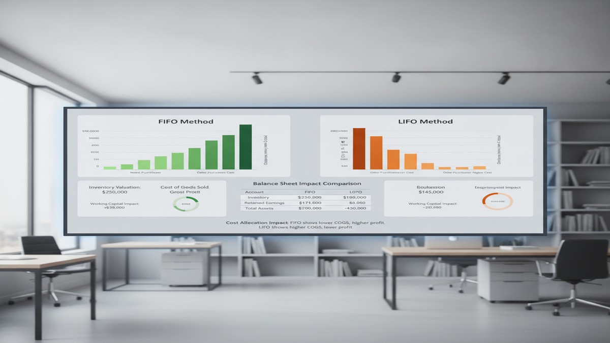
Business Central inventory costing methods FIFO vs LIFO comparison

When most finance teams implement Business Central, inventory costing defaults to FIFO. It’s the system default, it feels familiar, and no one on the implementation team flags it as a strategic decision. Then, 18 months into production, the conversation happens in the CFO’s office: your inventory balance sheet valuation has drifted significantly from what your tax accountant expected, your working capital metrics look different than they did under your legacy system, and your auditors are asking uncomfortable questions about whether the method you’re using actually aligns with your declared accounting policy.

This scenario repeats across organizations that underestimate the costing method decision as a finance strategy choice rather than a technical configuration. The truth is that your selection of FIFO, LIFO, weighted average, standard, or specific costing in Business Central ripples through your financial statements, your tax position, your working capital calculation, and your audit trail in ways that matter far more than most implementation teams realize.

## Why the Costing Method Choice Actually Matters to the Bottom Line

Business Central’s inventory costing method determines which purchase prices flow into your cost of goods sold and which prices remain sitting in inventory on your balance sheet. This distinction seems technical, but the financial impact is substantial. When prices rise, different costing methods produce radically different results: one method increases your reported profits and tax liability, another decreases both, and a third lands somewhere in between. The method you choose today locks in a path for your working capital metrics, your borrowing capacity, and your tax strategy for years to come.

Beyond the numbers, the costing method choice also determines how flexibly you can adjust costs after posting, whether you can back-date transactions without recalculating everything downstream, and how much discipline you need from your inventory and purchasing teams to keep the GL in sync with your ledger. Some methods are forgiving when you discover a $5,000 invoice weeks after posting; others force you to recalculate thousands of ledger entries and reconcile your entire inventory GL account.

## FIFO: The Default That Often Feels Wrong Under Inflation

First-In, First-Out assumes that the oldest items purchased are the first ones sold. When prices are stable or declining, FIFO produces intuitive results. When prices rise, FIFO increases your reported inventory value and profits, which sounds good until tax day arrives and your tax liability rises with it. In an inflationary environment, FIFO inflates your balance sheet. Your inventory looks more valuable, which helps you approach lenders and improves your current ratio. Your cost of goods sold stays lower, making gross margins look better. But your reported profit grows, and so does your tax bill.

FIFO is also straightforward to reconcile. Business Central tracks which purchase transactions were consumed in which sales, so tracing cost flows back to specific purchase invoices is relatively transparent. If you discover a cost error in a purchase invoice, you can correct it without triggering a cascade of recalculations across the entire inventory GL. These operational benefits make FIFO the path of least resistance for many finance teams.

The constraint worth noting: once you set an item to FIFO in Business Central, you cannot change to a different costing method if any ledger entries exist for that item. This lock-in effect means your initial FIFO choice is likely permanent for years, even if business conditions shift.

## LIFO: The Tax Advantage with Regulatory Complications

Last-In, First-Out assumes that the most recently purchased items are sold first, which produces the opposite financial effect of FIFO. In an inflationary environment, LIFO decreases your reported profits and tax liability, which is why LIFO became popular during high-inflation eras as a way to reduce tax burden. Your cost of goods sold rises faster, your gross margin shrinks on paper, and your reported profit falls, which lowers your tax bill.

The catch is significant: LIFO is disallowed in many countries and regions outside the United States. If your organization operates internationally or plans to expand outside the US, LIFO creates compliance complications and audit friction. Some jurisdictions view LIFO as a method that artificially depresses profit, and regulators restrict or disallow its use entirely. For this reason, LIFO is increasingly rare in global organizations, even though it retains tax appeal in the US market.

## Weighted Average: The Middle Ground for Volatile Costs

Weighted average costing calculates a single average unit cost at a defined interval (daily, weekly, monthly, quarterly, or per accounting period). Every item consumed during that period uses the same average cost. This method produces results that fall between FIFO and LIFO, making it a reasonable choice when your product costs are volatile or you have mixed, homogeneous inventory such as chemicals, raw materials, or commodities where tracing individual purchase costs to specific sales is impractical.

The operational trade-off with weighted average is important: if you back-date a transaction, Business Central must recalculate all affected ledger entries and inventory GL entries within that averaging period. A single invoice correction that appears weeks after posting can trigger a recalculation wave that touches hundreds of inventory transactions. This recalculation risk makes weighted average less attractive in environments where posting errors surface late or where regular transaction corrections are common.

## The Real Decision Framework: What Finance Leaders Should Actually Evaluate

Selecting your costing method should be driven by three distinct questions, not by which method your legacy system used or which option appears first in the setup wizard.

First, what is your product cost environment? If product costs are stable or predictable, FIFO is operationally clean. If your costs are volatile and inventory is homogeneous, weighted average is more defensible. For highly valued, easily identifiable items, specific costing gives you exact cost tracking.

Second, what is your tax and financial reporting strategy? If you want to minimize tax liability in an inflationary environment, LIFO appeals. If you want to maximize reported profits and borrowing capacity, FIFO serves that goal. If you want a neutral middle ground that doesn’t swing too far either direction, weighted average is stable. This decision is not a technical question; it is a finance strategy question that should involve your tax accountant and CFO.

Third, what are your regulatory and audit constraints? If you operate globally, LIFO creates complications. If your auditors have strong opinions about industry-standard methods, align with those expectations upfront. If your working capital and cash flow metrics are tightly monitored by lenders, verify that your costing method choice aligns with debt covenant calculations.

Once these three questions are answered, the technical choice becomes clear.

## Common Mistakes That Surface After Cutover

Finance teams frequently discover problems with their costing method choice only after cutover has been running for months. One common mistake is defaulting to FIFO because the implementation team knew no better, then realizing too late that your tax strategy would have favored weighted average or that your auditor expected a different method. Another frequent issue is underestimating the back-dating problem with weighted average, only to discover months later that regular cost corrections trigger massive recalculation waves that destabilize your GL.

A third mistake is failing to ensure that your Dynamics purchasing and inventory teams understand the costing method you selected. If your team does not know that you have chosen LIFO, for example, they may manage inventory in a way that contradicts LIFO’s assumptions, making your GL reconciliation substantially harder and your audit trail less defensible.

## Resetting the Choice Requires Planning

If you discover six months after cutover that you selected the wrong costing method, reversing the decision is expensive and disruptive. The technical constraint is absolute: you cannot change an item’s costing method if ledger entries exist. Resetting requires either creating new item numbers and migrating open inventory to those new items, or conducting a full inventory revaluation and GL restatement. Both paths are operationally messy and often require auditor involvement to ensure the transition is defensible.

For this reason, getting the choice right upfront is worth the investment of time and expert input before cutover.

## The Real Impact: Working Capital and Strategic Positioning

The costing method you choose in Business Central is not a technical detail to delegate to the implementation team; it is a financial strategy decision that affects your reported working capital, your tax position, and your balance sheet strength for years to come. FIFO inflates your inventory value and profits during inflation, making your balance sheet look stronger to lenders but increasing your tax bill. Weighted average cushions you against cost volatility but exposes you to recalculation risk. LIFO minimizes taxes but creates regulatory complications.

Organizations that treat the costing method choice as a strategic decision, led by their CFO and tax accountant rather than by the technical implementation team, avoid costly reversals after cutover and build a Business Central GL that supports their actual financial and tax strategy. Routeget Technologies helps finance and operations teams make this strategic choice before implementation, ensuring that your Business Central configuration aligns with your working capital goals and tax objectives from day one.

The choice you make now will shape your financial statements for years. Make it deliberately.

—

#BusinessCentralInventory #InventoryCosting #WorkingCapital #BusinessCentralFinance #FIFOvLIFO #CFOStrategy #DynamicsFinanceOps #FinancialAccounting #CostAccounting #BusinessCentralCore

Finance team analyzing Business Central inventory valuation in office

About Routeget Technologies: Routeget Technologies is a Microsoft Dynamics consulting firm helping enterprise and mid-market organizations implement, optimize, and extend their Microsoft technology investments. Our teams combine deep technical expertise with business advisory experience to deliver implementations that drive operational efficiency and financial impact.

Intercompany Elimination Automation in Dynamics 365 Finance: The Journal Entry Trap Most Finance Leaders Miss

Finance operations team reviewing intercompany transactions

Opening Hook

You’re three weeks away from quarter-end close. Finance has forty intercompany transactions in the queue: payables between subsidiaries, recharges for shared services, allocation of corporate expenses. Your team has been manually creating elimination entries in Dynamics 365 Finance for two years now, checking each one against the subledger balances to make sure matching transactions offset properly. It works, but it’s a manual gauntlet—and every quarter, at least one entry gets posted twice, or one side doesn’t match the other, forcing a restatement. The real question isn’t whether you can automate it. It’s why you haven’t, and what you’re risking by waiting.

Intercompany elimination automation is one of those finance capabilities that sits between the realm of “obvious good idea” and “surprisingly complicated to implement.” Most organizations running Dynamics 365 Finance intend to automate it. Many skip it because the setup looks straightforward until you actually try to accommodate the real-world variations in how subsidiaries actually transact with each other. The result is that finance teams at medium and large enterprises spend days each close period on what should be a single-click process, and they accept monthly restatements as a cost of doing business.

The problem isn’t the tool. It’s the gap between what the elimination process *should* do and what most companies configure it to do.

Why Elimination Automation Fails in Practice

Intercompany elimination transaction flow diagram

Dynamics 365 Finance includes native intercompany elimination capabilities. You can set up elimination rules, run a batch process, and create the offsetting journal entries automatically. In theory, this solves the manual-entry problem. In practice, most finance teams who build this end up abandoning it or working around it because the actual requirements are messier than the standard feature handles.

The standard elimination process works like this: define a rule (for example, “eliminate all transactions between subsidiary A and subsidiary B”), run the process, and Finance creates an elimination entry that offsets the amounts on both sides. Clean. Logical. Doesn’t work for half your transactions.

Consider what actually happens at close time. You have intercompany payables where subsidiary A owes subsidiary B for consulting services. You have expense allocations where the parent company charged subsidiaries for IT overhead. You have intercompany sales that aren’t yet invoiced, sitting as accrued revenue. You have currency revaluation differences on intercompany balances. You have partial payments that leave hanging balances. You have transactions posted in different legal entities with different chart-of-accounts structures, so the elimination account on one side doesn’t perfectly mirror the elimination account on the other.

Standard elimination rules assume bilateral, matching transactions in symmetrical account hierarchies. Your actual data looks nothing like that. So when you run the elimination batch, you get partial results, exceptions, and holes you have to patch manually. The bottleneck doesn’t disappear; it just shifts from “enter elimination entries” to “fix elimination exceptions.”

Finance leaders often respond to this by either (a) maintaining manual entries anyway because they understand exactly what’s being eliminated, or (b) accepting that some intercompany balances don’t get eliminated and building manual reconciliation into the close checklist. Both options are expensive. Both hide the problem behind process discipline rather than solving it.

The Core Configuration Trap

The most common failure point is account-matching logic. Dynamics 365 Finance’s elimination feature requires you to specify which accounts on one side of the transaction pair with which accounts on the other side. This sounds straightforward: payables account 200100 on the subsidiary pairs with revenue account 400200 on the parent. For a multi-subsidiary enterprise, you end up with dozens of pairing rules, each of which assumes the same chart-of-accounts structure exists in every legal entity.

But most organizations don’t have symmetrical chart-of-accounts structures across subsidiaries. One subsidiary might use a three-digit cost center code as part of its account number; another uses a six-digit project code. One subsidiary’s chart reflects its regulatory requirements; another reflects its parent’s reporting structure. When you try to force a uniform pairing rule across this, the automation fails on the exceptions—and the exceptions are where your intercompany risk actually lives.

The second configuration trap is elimination method selection. Dynamics 365 Finance offers three elimination methods: by elimination account, by elimination rules, and by source dimensions. Many teams choose by elimination account because it sounds simpler: just specify the account number that identifies an elimination entry, and the system will eliminate matching balances. This works if every intercompany transaction is coded to the same elimination account. It fails the moment transactions are coded to different accounts based on business unit or transaction type, which is what most accounting policies actually require.

A third trap, often overlooked during implementation, is timing. The elimination process doesn’t recognize transaction reversals. If subsidiary A reverses an intercompany invoice in one period and reissues it in the next, the elimination logic might net them in one period (correctly) but not eliminate the new entry in the next (incorrectly). If you have accrual entries that roll forward, the system doesn’t know whether an accrual has been settled or not. You end up eliminating transactions that shouldn’t be eliminated, or leaving open balances that should have been cleared.

What Actually Works: The Approach That Finance Leaders Should Use

The finance teams with the most reliable elimination processes don’t rely on the standard feature to do all the work. Instead, they use Dynamics 365 Finance’s elimination tools as a framework, but they layer on additional validation and semi-automation. Here’s the pattern:

First, establish elimination rules that cover your high-volume, repetitive transactions. These are usually the 70 or 80 percent of intercompany activity that follows a consistent pattern: standard intercompany invoicing, allocated expenses, routine recharges. For these, the elimination batch process should work cleanly. Document what these rules eliminate, down to the account level and dimension combinations.

Second, build a separate process for exception handling. Run the elimination batch, but don’t post the results immediately. Export the elimination entries to Excel or a Power BI model, and validate them against your subledger balances before posting. Check that every elimination entry has a matching transaction on both sides of the elimination. Check that no entries are created for reversal transactions or accruals that should roll forward. This step takes time, but it’s a single review pass instead of forty manual entries, so it’s still a win. It also creates an audit trail for your external auditors.

Third, identify which intercompany transactions or balance types require manual elimination because they’re too irregular for the standard process. These might be settlement-in-progress balances, partial intercompany payments, or transactions that cross subsidiaries with fundamentally different chart structures. Document these explicitly. Don’t pretend the automation covers them. Instead, build a checklist that the finance team follows at close time to ensure these balances are explicitly reviewed and eliminated if appropriate.

Fourth, if your organization is running Dynamics 365 Finance with Power Automate or has development resources, invest in a custom validation flow. The flow should read the pending elimination entries, compare them to the underlying subledger transactions, check for matching invoices or supporting documentation, and flag entries that don’t pass basic reasonableness checks. This isn’t fully automatic elimination, but it’s a guardrail that catches the most common errors: duplicated entries, reversed entries posted as new eliminations, and account mismatches that slipped through the configuration.

The Business Case for Getting This Right

Finance organizations that automate 80 percent of intercompany eliminations and tightly control the remaining 20 percent typically see close cycles compress by two to three days. They reduce restatements for intercompany errors to nearly zero. They cut the finance team’s close-period overtime significantly. They have a documented process that external auditors can review with confidence.

But the real benefit is visibility. When intercompany eliminations are systematized, not manual, you actually know which transactions were eliminated and why. You have an audit trail. You can run analytics on intercompany activity and see patterns: which subsidiaries have the most outstanding intercompany balances, which transaction types take longest to settle, where cash is actually stuck in the system. That visibility drives better working capital management and faster cash conversion.

The risk of not doing this isn’t just operational. If your finance team is doing intercompany eliminations manually, you’re relying on individual judgment calls about what to eliminate and what to leave open. That’s fine until someone new joins the team, or someone leaves, and the institutional knowledge walks out the door. You end up with intercompany balances that neither the subsidiary nor the parent fully understands. You run into issues at audit time or during a consolidation review that force a restatement.

Getting Started

If you’re currently doing intercompany eliminations manually in Dynamics 365 Finance, your first step is to stop trying to fully automate them immediately. Instead, audit what you’re actually eliminating each month. Document the transactions, the accounts involved, the business rationale. This gives you the blueprint for what the automation should cover versus what requires manual review.

Build the elimination rules in a test environment first, and run them against three months of historical data. Don’t post the entries. Instead, compare what the system generated against what your finance team actually eliminated in those three months. Identify where the automation missed transactions or created incorrect entries. Fix the configuration. Repeat.

Once the automation covers the repetitive 80 percent cleanly, document what’s left as exception handling. Document the account pairing rules so that whoever is managing the process next year—or five years from now—understands why the automation is configured the way it is.

If you have the resources, layer on a Power BI dashboard or a Power Automate flow that validates elimination entries before posting. Even a simple check that counts invoices on both sides of the elimination catches most errors.

The close process is where finance leaders are usually most stretched during the month. Taking even two days off your close cycle is worth the implementation effort.

About Routeget Technologies

Routeget Technologies has spent years helping mid-market and enterprise finance organizations streamline their period-close processes in Dynamics 365 Finance. Intercompany elimination automation is one of the first things we look at during an implementation review because it’s one of the highest-return-on-effort improvements available. If your current close process is still mostly manual, we can help you audit what’s actually happening, design an elimination configuration that works for your subsidiary structure, and build the validation layer that keeps the automation reliable.


#IntercompanyElimination #DynamicsFinanceOps #FinanceAutomation #PeriodClose #ERPGovernance #FinanceTransformation #DynamicsFinance

AI Builder Document Intelligence: Why Your Finance Team Still Manually Keys 2,000 Invoices a Month

AI Builder Document Intelligence: Why Your Finance Team Still Manually Keys 2,000 Invoices a Month

For most large enterprises running Dynamics 365 Finance, accounts payable looks straightforward on paper: invoices arrive, they get matched to purchase orders, approvals happen, payments post. In practice, the first step is where the actual work lives.

An average mid-market organization processes 2,000 to 5,000 invoices per month across dozens of vendors. Each arrives in a different format, with fields in different positions, sometimes with missing data. A finance team that tries to automate this early usually concludes it is not worth the engineering effort. The result is a process that remains almost entirely manual: an AP clerk opens an email, scans an attachment, reads the invoice line by line, and keys data into the ERP by hand.

The financial impact compounds invisibly. A clerk processes around 30 to 50 invoices per day. That is 8 to 10 minutes per invoice of pure data entry, plus rework for errors. Across 2,500 monthly invoices at an average of 40 minutes per invoice, you have roughly 1,667 labor hours per month, or 8 to 10 full-time equivalent staff just feeding data into your ERP. The opportunity cost is real: those people are doing work machines could do better.

Intelligent document processing has existed for years, but it historically demanded custom machine learning expertise or vendor lock-in to specialized platforms. AI Builder changes that. It is a low-code intelligent document processing engine built directly into the Power Platform and accessible through Microsoft Dataverse. Using AI Builder’s document intelligence model, you can teach a system to extract data from invoices, POs, or receipts, and have that extracted data automatically flow into Finance and Operations as journal entries, vendor invoices, or line items, without custom code or a separate platform.

The catch is that most implementations get the architecture wrong, deploy too early, or do not think through the business case clearly enough to justify the investment.

What AI Builder Document Intelligence Actually Does

AI Builder’s document intelligence model learns patterns from example documents. You supply 5 to 100 sample invoices, mark the specific fields you want extracted (invoice number, date, line item amounts, vendor name, cost center), and AI Builder trains a model. Once trained, it processes new invoices and extracts those fields with a confidence score for each value.

The extraction outputs structured data as JSON, which flows into Power Automate, passes to Dynamics 365 through REST APIs, or writes directly to Dataverse tables. You can build an approval workflow where extracted data is reviewed by humans, corrections are made if confidence scores are low, and once approved, the invoice posts without manual rekeying.

The critical limitation: AI Builder solves data entry, not the entire AP transformation. It does not solve the three-way match or reconciliation of discrepancies between invoice amounts and actual receipts. If invoices regularly have billing errors or missing line items, AI Builder will extract those discrepancies accurately, but human approval workflows are still required to investigate.

AI Builder also assumes reasonably stable vendor populations. If vendors send different invoice formats month to month, or you have 200 vendors across five countries with different field positions, you may need multiple models or a more flexible extraction architecture.

The Actual Implementation Costs

The common mistake is to assume that because AI Builder is “low code,” implementation cost is proportionally low. It is not.

Training a single AI Builder model requires deciding which fields are worth extracting, building a training set, and determining how much format variance the model needs to handle. You cannot build a generic model across all vendors. You have to scope it precisely. Multiple vendor formats require multiple models or accepting lower confidence scores and higher downstream rework.

The real cost sits in the integration layer. You need a Power Automate flow that ingests documents, calls the AI Builder model, handles extracted data, performs validation and enrichment (cost center lookups, amount threshold checks, purchase order verification), and posts data into Dynamics 365 Finance. That flow needs error handling, logging, and exception routing for human review. You also need to decide where documents come from: email, OneDrive, a vendor portal. Each source requires a different ingestion pattern.

A medium-complexity invoice processing automation project involving 5 to 10 major vendors, one AI Builder model, and robust Power Automate orchestration typically runs 6 to 12 weeks, roughly 300 to 600 professional services hours. At 200 USD per hour fully loaded, that is 60,000 to 120,000 USD. AI Builder licensing is usage-based at roughly 0.01 to 0.02 USD per page. An organization processing 2,500 invoices per month with 3 pages each processes 90,000 pages annually, costing 900 to 1,800 USD in consumption.

But labor savings are substantial. Saving 1,667 hours per month at 45 USD per hour fully loaded equals 75,000 USD monthly, or 900,000 USD annually. Even if net savings are 70 percent of that due to exception handling and ongoing overhead, you still have 630,000 USD in annual labor savings against a 120,000 USD implementation cost. Payback happens in 2 to 3 months.

Those numbers are achievable if, and only if, you have a focused vendor population, reasonably consistent invoice formats, and a clear baseline for how much time the manual process actually consumes. Many organizations skip that baseline measurement, build the system anyway, and then cannot measure whether it actually saved time.

Common Failure Modes

The most common failure is misalignment on scope. Finance wants to automate “all invoices.” Engineering builds one model for all vendor formats. The model trains on 50 random invoices from 20 different vendors. When it encounters a new vendor invoice, confidence scores are low, and the entire pile ends up in the exception queue. The fix: scope tightly. Start with 3 to 5 major vendors representing 40 to 60 percent of volume. Get those working first. Add additional vendors only after the core extraction pipeline is mature and stable.

The second failure is underestimating validation and enrichment workload. Once you extract data, you need to validate it. Does the date make sense? Is the vendor in the master list? Is the amount within normal range? If any check fails, the invoice needs review. Without a validation layer, you have not saved labor; you have shifted it from data entry to exception handling.

The third failure is publishing to Dynamics 365 without handling master data dependencies. A vendor invoice requires valid vendor master records, cost centers, and often purchase order references. Incomplete or inconsistent vendor master data means extraction works perfectly but posting fails because the vendor cannot be resolved. This shows up as an AI Builder problem when implementation teams do not plan for data quality prerequisites upfront.

When AI Builder Works

The use cases with clear ROI are relatively specific.

The strongest case is a company with a stable vendor population where the top 10 to 20 vendors represent 70 percent of invoice volume and use consistent invoice formats. Train one or two models for those top vendors, automate their extraction entirely, and you have converted 70 percent of invoice volume from manual to automated. The remaining 30 percent stay manual, but you have cleared the decks of high-volume repetitive work.

The second strong case is an ERP migration where the existing system has data entry backlogs. Using AI Builder to accelerate historical invoice loading during migration can meaningfully shorten timelines. Post-migration, you keep the system running for ongoing automation.

The third case is significant localization requirements, where invoices come from subsidiary companies in multiple countries and languages. AI Builder’s multilingual capabilities handle non-English documents, so you can build a single orchestration layer that routes invoices by language, extracts data consistently, and maps that data to the right cost centers based on geography.

Measuring Before Committing

Before starting, measure three things.

First, measure current invoice processing with precision. How many invoices per month? Average time per invoice from receipt to posting, broken down by task (data entry, validation, research, approval, posting)? Error rate and rework volume? These numbers should come from actual time tracking, not estimates.

Second, identify scope. Which vendors represent the top 50 percent of volume? Are their formats consistent month to month? If you extracted 20 sample invoices from your top 10 vendors, how much variation would you observe in field positions? This informs whether you need one model or multiple models.

Third, confirm you have people and tools in place. AI Builder handles extraction, but you still need a Power Automate designer, a Dynamics 365 developer, and ongoing operational ownership for the flow. If you would need to hire these resources, that cost belongs in the implementation budget.

With those measurements, the business case becomes concrete. You can calculate labor savings per month against implementation cost and decide with confidence whether the project pencils out.

AI Builder document intelligence is not a panacea for AP efficiency, but in focused scope with stable vendor populations and consistent invoice formats, it solves a real problem that costs most large enterprises hundreds of thousands of dollars per year in pure human labor. The implementation requires clarity on scope, attention to data quality, and realistic expectations about exception handling. But for the right use case, the ROI is compelling enough to build into your Dynamics 365 Finance roadmap.


Hashtags: #AIBuilder #DocumentIntelligence #InvoiceProcessing #DynamicsFinance #FinanceAutomation #DynamicsFinanceOps #RPA #PowerPlatform

Dynamics 365 Tax Calculation Migration Gets an Automated Tool. It Still Needs a Reviewer.

Finance systems analyst reviewing Dynamics 365 tax configuration data on a monitor

A finance solution architect I spoke with recently put the choice in blunt terms: her team’s Sales Tax configuration has worked reliably for nine years, and nobody wants to touch it, but Microsoft has made it clear that Advanced Tax Calculation, not the legacy Sales Tax module, is where indirect tax functionality in Dynamics 365 Finance is actually heading. That tension shows up in nearly every conversation about a Dynamics 365 tax calculation migration: teams know the destination, but re-keying years of tax codes, tax groups, and jurisdiction rules by hand is not a project anyone volunteers for. With the 2026 Wave 1 release, Microsoft shipped a preview feature aimed at closing that gap, and it deserves a close technical look before anyone assumes it turns migration into a one-click event.

What the Tax Calculation Migration Tool Actually Moves

The feature, officially called “Automate tax feature creation based on tax master data,” lives in Globalization Studio under Tax Calculation, and it is activated through a Feature Management flag rather than being on by default. Once enabled, it reads a legal entity’s existing sales tax master data (tax codes, sales tax groups, and item sales tax groups) and builds an equivalent Tax Calculation feature version from it, reusing the reference data rather than asking anyone to redefine it from scratch. It also maps general ledger parameters that previously lived at the legal entity level, reverse sales tax on cash discount, whether cash discount is deducted before tax calculation, and whether cash discount is calculated on an amount including tax for both customers and vendors, onto their equivalent Tax Jurisdiction Parameters in the new model. Tax code origin settings translate as well: percentage of gross amount becomes “By Gross Amount,” percentage of net amount becomes “By Net Amount,” percentage of margin becomes “By Margin,” and so on through amount-per-unit and tax-on-tax origins.

Finance systems analyst reviewing Dynamics 365 tax configuration data on a monitor

That mapping table matters more than it looks. Anyone who has manually stood up Advanced Tax Calculation before knows that recreating tax jurisdiction parameters and origin rules correctly, across dozens of tax codes, is where most implementation hours actually go. Automating that translation, even in preview, removes a meaningful chunk of the grinding part of the work.

Where the Automation Runs Into Real Constraints

The tool is scoped to one legal entity at a time, and it requires the operator to be signed into the correct legal entity before starting the process from the Tax Data Migration button in Globalization Studio. It is also explicitly unavailable for Brazil and India legal entities, so multinational rollouts will need a separate manual path for those jurisdictions regardless of how well the automated tool performs elsewhere.

Two hard limits are worth flagging before anyone schedules migration work around this tool. Tax code names are capped at ten characters in the target model, and when a naming conflict forces the tool to create a variant, it truncates the original name and appends a numeric suffix, so “Test123456” becomes “Test1234_1.” Separately, if the combined character length of the tax codes attached to a single tax group or item tax group exceeds 1,000 characters, the migration for that group fails outright with an explicit error rather than a partial or degraded result. Neither limit is exotic for a small implementation, but a legal entity that has accumulated hundreds of tax codes over a decade (which describes a fair number of established Dynamics 365 customers) can hit the 1,000-character ceiling without anyone realizing it was a live risk until the process stops.

Reading the Variant Logic Correctly

Tax code variants deserve particular attention because the tool’s behavior here is deterministic in outcome but not in labeling. When the same tax code is assigned to more than one tax group with different parameters, for instance a code marked Exempt in one tax group and configured with Use Tax enabled in another, the migration creates separate variants, such as Test10, Test10_1, and Test10_2, to preserve both configurations rather than collapsing them into one and losing data. The parameter mappings themselves come through correctly, but which suffix lands on which variant is not something to assume from naming alone. Microsoft’s own documentation notes the suffix order isn’t guaranteed to follow a predictable pattern. A reviewer needs to open each variant and check its assigned tax group and parameters directly, rather than trusting that _1 always corresponds to the first tax group alphabetically or chronologically. Skipping that verification step is the most likely way a migration looks clean in testing and then produces a wrong tax determination on a specific transaction type in production.

Cash discount handling is the other area that needs a second look rather than a rubber stamp. Because the legacy model sometimes allowed cash discount settings to diverge between the general ledger parameters and individual sales tax groups, the migration surfaces a warning wherever it detects that discrepancy instead of silently picking one value. That warning is not cosmetic. It flags a real business decision, specifically which cash discount behavior should win going forward, that the automation correctly declines to make on its own.

Two enterprise IT professionals reviewing a tax migration report and dashboard

What This Means for a Dynamics 365 Tax Calculation Migration Project Plan

None of this changes the fundamental recommendation: this is a preview feature, and Microsoft’s own guidance is explicit that it is not intended for production use yet. Treat a run of the tool as generating a strong first draft of the target configuration, not a finished migration. The realistic project plan looks like importing the latest tax configuration through Electronic Reporting, enabling the preview flag in Feature Management, running the tool against a non-production legal entity, and then working through a defined review checklist. That checklist should confirm every tax jurisdiction parameter actually matches current business intent rather than just what the legacy setup happened to contain, trace every tax code variant back to its correct tax group assignment, resolve every cash discount warning as a deliberate decision, and check the default rounding method, which the tool sets to Ordinary regardless of what a given legal entity may actually need. There is also no incremental sync: if master data changes after a feature version is created, that version does not update itself, and the team has to decide whether to regenerate a new version or maintain the delta by hand.

For a solution architect scoping this work, the honest framing is that the tool changes where implementation hours go rather than eliminating them. It removes most of the manual re-entry burden and replaces it with a structured, checklist-driven review, which for a data set of any real size is still a substantially better trade than doing both the entry and the review from a blank slate. Firms that have run tax configuration projects on both the legacy and Advanced Tax Calculation models, Routeget Technologies among them, tend to build that review checklist into the statement of work up front, specifically because the tool’s own limitations (character caps, entity-by-entity scope, and the Brazil and India exclusions) are exactly the details that get missed when a migration is treated as a single automated step instead of a reviewed one.

Teams planning a Dynamics 365 tax calculation migration over the next few Wave releases should watch for this feature’s move from preview to general availability, since GA typically brings expanded country coverage and, ideally, an incremental update path. Until then, the tool is genuinely useful for what it is: a way to stop re-keying tax codes by hand and start reviewing a generated draft instead. That is a real improvement in a project that used to have no shortcut at all, even if it is not yet the fully automated migration some teams are hoping for.


#TaxCalculationService #DynamicsFinanceOps #GlobalizationStudio #ERPTaxCompliance #TaxAutomation #FinanceTransformation

Financial Tags Finally Cover Purchase Order Invoicing in D365 Finance 10.0.49. Ledger Settlement Still Won’t Match Half of Them.

Finance professional reviewing a general ledger reconciliation dashboard with matched and unmatched transaction indicators

A controller running month-end reconciliation on a clearing account in Dynamics 365 Finance has a specific, recurring headache: the debit side of a transaction carries a purchase order number as a financial tag, the offsetting credit side does not, and the ledger settlement engine treats the two lines as unrelated even though anyone looking at the source documents can tell they belong together. Until version 10.0.49, this was a permanent structural gap rather than an occasional configuration mistake, because financial tags on purchase order invoicing simply did not exist as a supported scenario. Sales order invoicing got tag support years earlier. Purchase orders did not, which meant any finance team using tags to track PO references through the vendor side of the ledger was stuck writing the number into a description field or a financial dimension never designed to hold it. That gap closed with 10.0.49, and the fix is worth understanding in detail, because the parts of financial tags that already worked reasonably well are not the parts that are going to trip up the teams adopting this now.

What Financial Tags Actually Are, and Why the PO Gap Mattered

Financial tags are not a new concept in Dynamics 365 Finance. Introduced in version 10.0.16, they give a legal entity up to twenty user-defined fields that attach supplementary reference data directly to a general ledger voucher line, things like an external invoice number, a customer name, or a payment reference, without that data ever touching a subledger table or a financial dimension. That distinction matters more than it sounds. Financial dimensions were built for reusable, hierarchical, reportable categories: cost center, department, business unit. A purchase order number is none of those things. It is a single-use reference that exists to answer one question later: which document generated this line. Forcing that kind of data into a dimension structure bloats the dimension combination table and adds no analytical value, since nobody is running a financial report grouped by PO number. Tags were built specifically to hold this lower-reusability data cleanly, and by the time sales order invoicing gained tag support, most finance teams using the feature had already built tagging conventions around customer-side transactions. Vendor-side transactions were the obvious next step, and the 10.0.49 release finally delivers it, gated behind a feature called Enable financial tags for purchase order invoicing that sits alongside the equivalent, longer-standing sales order feature in Feature management.

Where the Real Work Starts: Ledger Settlement Matching

The reason this release deserves more than a changelog mention is that financial tags do something beyond passive record-keeping. They can serve as match criteria inside ledger settlement, the process finance teams use to pair debit and credit lines on clearing, prepaid, accrual, and other temporary accounts and mark them as settled. In principle, tagging both the AP-side and AR-side (or intercompany) legs of a transaction with the same PO reference should make settlement close to automatic: the engine finds the matching tag values and clears the pair. In practice, three specific failure patterns show up constantly, and none of them produce an error message that tells you what actually happened.

Close-up of hands reviewing a voucher transaction table with reference and status columns on a laptop

The first is the mismatched-side problem this article opened with. If the debit line carries a tag value and the credit line does not, or the two sides carry different values because they were entered by different people at different points in the process, settlement will not treat them as a match. There is no fuzzy matching here. The comparison is exact, and a trailing space or a different capitalization convention is enough to break it. The second is a timing problem specific to any organization adopting purchase order tagging now rather than at initial go-live: transactions posted before the feature was activated simply have no tag value on the line at all, which means every open item predating the 10.0.49 upgrade needs a separate remediation pass before it can participate in tag-based settlement. You cannot retroactively tag a posted voucher through the transaction UI; the supported path is the internal voucher data edit function, gated behind the Allow edits to internal data on general ledger vouchers feature, and it needs to run as a deliberate cleanup project, not something a settlement clerk discovers mid-close.

The third failure mode is the one that catches experienced admins off guard, because it involves a change that looks harmless. Tag labels can be renamed at any time without affecting already-posted data, which is a genuine convenience when a naming convention needs to evolve. But posted voucher lines retain whatever tag value was in effect at posting time, and if two lines that logically belong together were posted before and after a rename, or against two tags that were later consolidated under one label, the underlying stored values can diverge from what the current tag configuration implies, and settlement compares stored values, not current labels. A team that renamed a tag mid-quarter for good reasons can end up with a batch of open items that look identical in the UI but fail to match, and the only way to find out why is to pull voucher transactions against the general journal account entry table (not the financial tags table, which only exposes generic Tag01 through Tag20 labels and hides which business tag they actually correspond to) and compare raw values line by line.

Configuration Details Worth Getting Right Before You Enable the Feature

Beyond the settlement-matching behavior, a few configuration decisions are easy to get wrong on the first pass and expensive to unwind later. The delimiter used to separate tag values in General ledger parameters cannot be changed once set, so it is worth choosing a character your reference data will never plausibly contain, not just one that looks clean in a demo. Validation is optional by default even for list-type tags; as of 10.0.44, Fixed list and Fixed custom list value types exist specifically to prevent free-text drift, and for any tag that will be used as a settlement match key, that validation should be non-negotiable rather than left at the default. And because tag configuration changes are cached at the user session level, a tag that was just activated or edited will not reliably show up for a user until they sign out and back in and, in stubborn cases, clear the usage data cache under user options; teams that skip this step and conclude a newly enabled tag “isn’t working” are usually looking at a caching artifact, not a configuration bug.

For a finance function evaluating whether to turn purchase order tagging on now, the sequencing that avoids the most rework is to finalize the tag definitions and delimiter first, apply fixed-list validation to anything that will drive settlement matching, activate the feature and confirm both sides of a representative PO-to-payment cycle post with identical tag values, and only then decide how far back to remediate historical open items rather than assuming the feature will somehow reach backward on its own. None of this diminishes what 10.0.49 actually fixes: a real, years-old asymmetry between how sales and purchase transactions could be tagged is gone. What it does not fix, and was never going to, is the discipline required to keep tag values consistent across two sides of a transaction that are frequently entered by different people, in different modules, at different times. Routeget Technologies has helped finance teams build that discipline into their close process rather than discovering the gap during an audit, and the pattern is consistent enough across clients that it is worth planning for before enabling the feature rather than after the first failed settlement run.


#FinancialTags #DynamicsFinanceOps #LedgerSettlement #PurchaseOrderInvoicing #GeneralLedger #ERPReconciliation

Dataverse Long-Term Retention Can Cut Your F&O Storage Bill in Half. It Doesn’t Keep Your Encryption Key.

IT and finance leaders reviewing a Dataverse storage capacity dashboard in a boardroom

A CFO reviewing next year’s Power Platform renewal usually finds the same line item growing faster than anything else on the invoice: Dataverse database capacity. For a Dynamics 365 Finance and Supply Chain Management customer with a few years of general ledger, tax, inventory, and sales order history behind it, that growth is not a mystery. Transactional tables in F&O apps do not shrink on their own, and every fiscal year adds another layer of records that almost nobody queries but that the platform still has to store, index, and back up at full price.

IT’s answer to that problem usually arrives as a single line in a capacity review deck: turn on Dataverse long-term retention and archive the old transactions out of the live database. It is a real fix, and Microsoft’s own numbers back it up. But the conversation tends to stop there, before anyone asks the question a security or compliance lead should be asking, which is what happens to the encryption key protecting that data once it moves.

Why F&O Capacity Grows Faster Than the Budget Assumes

Dataverse long-term retention, sometimes shortened to LTR, lets an organization move inactive records out of live application tables into a separate, read-only retention layer that still lives inside Dataverse and is still governed by Microsoft Entra ID. For Finance and Supply Chain Management specifically, Microsoft currently supports archiving general ledger transactions, tax transactions, inventory transactions and journals, sales orders, and Commerce transactions this way. Attachments are explicitly excluded for now.

The financial case is straightforward once you see the compression numbers. Microsoft states that data moved into Dataverse long-term retention consumes roughly half the capacity of the same data sitting in a live table, and when the F&O-specific archive process goes a step further and migrates that data into history tables rather than leaving it only in retention, the history-table footprint can run closer to 30 percent below the original. At a commonly cited list price of roughly 40 dollars per gigabyte per month for Dataverse database capacity, an organization sitting on several hundred gigabytes of aging general ledger and inventory history is not looking at a rounding error. It is looking at a five- or six-figure annual number that a straightforward archive policy can meaningfully cut, without touching a single report a controller actually runs day to day.

That is the pitch that gets this feature onto a roadmap. It is also, on its own, an incomplete pitch.

What Dataverse Long-Term Retention Actually Does, and How Long It Takes

The mechanics matter for planning purposes, not just for understanding the technology. Microsoft’s documentation describes the F&O archive process as a sequence of stages: replication of records into Dataverse long-term retention, marking of records that meet the retention policy’s criteria, reconciliation to confirm every record made it across intact, and finally migration, where the data is moved into history tables and removed from the live application tables. Only after that full sequence completes does the capacity reduction actually show up in reporting, and Microsoft’s own timeline for that is seven to fourteen days depending on data volume, with archival jobs deliberately run at lower priority than normal application workloads.

There is a detail buried in that same documentation that tends to surprise architects who assume large-scale platform jobs run in parallel by default: they do not, here. Microsoft states plainly that the stages of the F&O archival process “run sequentially in the background.” If you are planning to archive several years of general ledger, tax, and inventory history in the same cycle, that sequencing, not the compression ratio, is what actually determines how long your capacity relief takes to land. A rollout plan built around a single “flip the switch and wait a week” assumption is usually wrong by a factor of several weeks once multiple table types and several years of backlog are involved.

None of that is disqualifying. It is simply the kind of operational detail that belongs in a project timeline, not a surprise a program manager discovers in week three.

The Encryption Question That Actually Changes the Decision

Close-up of a compliance professional reviewing an encryption key management interface on a laptop

Here is where the conversation should slow down before a decision gets made, particularly for regulated industries such as financial services, healthcare, government contracting, or any organization with a contractual or regulatory commitment to control its own encryption keys.

Microsoft Power Platform has moved through two generations of customer-controlled encryption. The older mechanism, generally referred to as bring your own key or BYOK, is now explicitly positioned by Microsoft as a legacy predecessor to the current customer-managed key, or CMK, model. That distinction is not cosmetic. Microsoft’s own migration guidance states that environments still running the legacy BYOK encryption model are locked out of a specific list of newer Dataverse capabilities until they migrate to CMK, and Dataverse long-term data retention is on that list, alongside elastic tables, Dataverse search, AI Builder, and several others. An organization that has not made the BYOK-to-CMK move simply cannot turn retention on yet.

For organizations evaluating the F&O-specific archive path directly, Microsoft’s own archive documentation adds a second, sharper detail. It states that customers using the legacy BYOK model should be aware that data moved into Dataverse long-term retention is encrypted with a Microsoft-managed key rather than the customer’s own key, and it recommends migrating to customer-managed key as a result. Read carefully, that is Microsoft telling its own customers that the encryption custody model can change the moment data crosses from a live table into the archive, unless the tenant has already completed the CMK migration first. It is worth noting that the guidance itself is not fully explicit about whether this applies only to tenants still on the older model or to every tenant regardless of current key configuration, and a security team relying on this feature for a compliance commitment should confirm the current behavior for their specific tenant and encryption configuration directly with Microsoft before treating archived data as covered by the same key custody guarantee as their live data.

For a business that markets its own data handling on the strength of customer-held encryption keys, whether to a regulator, an auditor, or a customer contract, that is not a footnote. It is a governance gap that needs to close before the capacity-savings project starts, not after an auditor asks where the archived general ledger data actually lives and under whose key.

Sequencing the Decision Correctly

The organizations that get this right treat Dataverse long-term retention as a governance initiative with a cost-savings side effect, not the other way around. That means confirming current encryption status first: whether the tenant is still on legacy BYOK, already on CMK, or using Microsoft-managed keys by default, since only the first case actually creates a conflict. It means building the CMK migration, if one is needed, into the project plan ahead of the retention policy rollout rather than in parallel with it, since Microsoft’s own guidance describes CMK migration as something that can happen without contacting Microsoft support, which removes one common excuse for delay. And it means setting expectations with finance leadership that the capacity savings materialize over a multi-week sequential process per table type, not overnight, so the budget conversation is not built on a timeline the platform cannot actually deliver.

We at Routeget Technologies have walked F&O customers through exactly this sequencing, and the pattern holds consistently: the technical archive configuration itself is the easy part. The harder, more valuable conversation is the one between IT, finance, and compliance about what “the data is still in Dataverse” actually means once the key protecting it is no longer necessarily the one the organization chose.

The capacity savings on a Dataverse long-term retention rollout are real, and for an F&O environment with years of transactional history, they are often large enough to justify the project on cost grounds alone. But the encryption question is not a technicality to resolve after the fact. It is the first question a CIO or CFO should ask before the retention policy goes live, and the answer determines whether this is a two-week configuration task or a multi-month project that starts with a key migration.


#DataverseRetention #CustomerManagedKey #BYOKMigration #DynamicsFinanceOps #ERPCostOptimization #CloudArchitecture